
Analytic methods of normality.
Skewness and kurtosis are two of the first four moments of a normal distribution. Both can be used to test the assumption of normality of a data distribution, although they are less widely used than other contrast pr graphical methods.
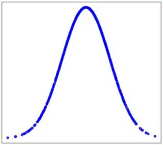
The normal distribution never ceases to amaze us with its beauty and harmony, as well as its simplicity.
A distribution so central to statistical inference is very easy to characterize, we just need to know its mean and variance (or the square root of the latter, the standard or typical deviation).
But that does not mean that all data series that follow a normal distribution are identical if we represent them graphically. They all have a similar bell shape, are more or less equally stylized, and also more or less symmetrical.
And why do I say “more or less”? Well, because, in real life, nothing and nobody is perfect, not even the normal distribution. Well, the standard normal distribution does meet the characteristics of a perfect normal distribution.
A standard normal distribution is characterized by having a mean equal to zero and a variance equal to one. It is usually represented as N(0,1). But, in addition, we can characterize it from its moments.
One moment… or better, four of them
Some of you may wonder what I mean by the moments of distribution. Let’s see it.
Statistical moments have nothing to do with time. Rather, they are inspired by moments in physics, which have to do with the mass centers of systems.
Here we are not dealing with masses, but with series of values that follow a given probability distribution.
The first moment is calculated as the sum of the values of the variable divided by the total number of values in the distribution. This, all of you who are still awake will have understood, is nothing more than the mean of the distribution.
To calculate the other moments we will use the sum of the differences of each value of the variable with respect to the mean of the distribution. The problem is that, since the distribution is symmetric, some differences will cancel each other out so that the average of the differences would be zero.
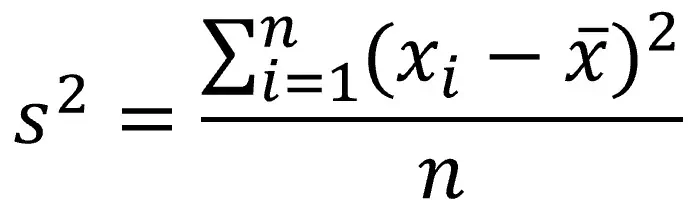
The solution to the problem of differences canceling each other out is to square them, making negatives to positive. By dividing this sum by the n of the distribution, guess what we get? In effect, the variance, the second moment. Here is the formula to see it more clearly:
If we continue playing with the differences and cube them, what do you think would happen? Well, we will calculate the average of the cube of the deviations of the values with respect to the mean, which would be the third moment of the distribution.
If we think a bit, we will soon realize that when we cube we no longer lose the negative signs.
In this way, if there is a predominance of negative values (the distribution has more values less than the mean) the result will be negative and, conversely, if values greater than the mean predominate, it will be positive (the distribution will be skewed to the right ).
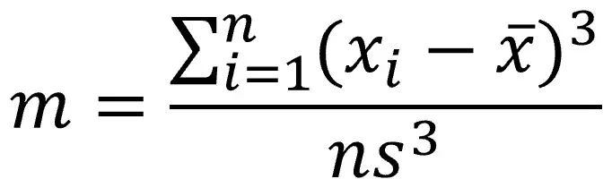
If we divide this average sum of differences cubed by the cube of the standard deviation, we will obtain the dimensionless version of the third moment of the distribution, which is none other than the index of symmetry or skewness of the distribution.
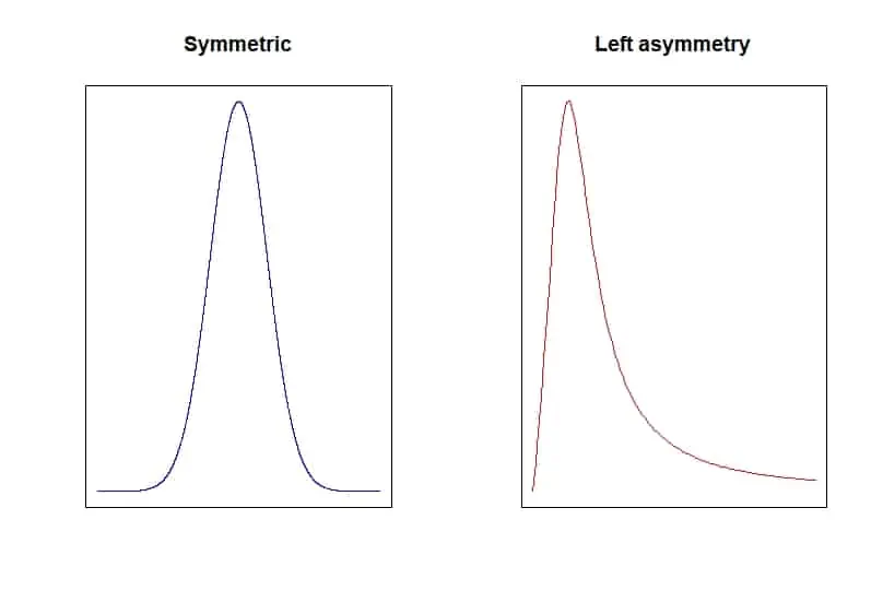
You can see in the first figure two examples of distribution, one of them symmetrical (figure on the left) and the other skewed to the right.
Finally, let’s go one step further and calculate the sum of the differences between each value and the mean raised to the fourth power and divided by the n of the distribution. This would be the fourth moment, which we can divide by the standard deviation raised to the fourth power:
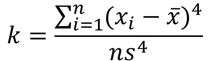
We thus obtain the dimensionless version of the fourth moment, known as kurtosis, which measures how pointed is the bell that forms the representation of the distribution.
At this point we have to make a clarification. The kurtosis of the standard normal distribution is equal to 3. For this reason, what is known as excess kurtosis is usually used, subtracting 3 from the formula:
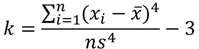
This is done like this, explained in a very simple way, to force the value of the kurtosis of the standard normal distribution to be 0.
This index indirectly indicates the amount of data in the distribution close to the mean. Thus, the higher the degree of kurtosis, the distribution will be more stylized and the tails will be lighter. And the other way around, with lower kurtoses, there will be less data around the mean and the tails will be heavier.
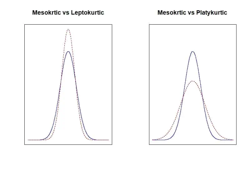
Based on this, we will say that the distribution is leptokurtic if it is very stylized (the values are very clustered around the mean). On the contrary, if the values are dispersed at the extremes, we will call it platykurtic (it will be less pointed) and, if neither one thing nor the other, we will speak of a mesokurtic distribution.
In the second figure that I attach you can compare a normal mesokurtic distribution with a leptokurtic (left) and a platykurtic (right).
The moments of the standard normal distribution
We have already mentioned the values of the first two moments. A standard normal distribution is one with mean 0 and variance 1: N(0,1).
Thanks to the perfection of the standard normal distribution, its symmetry index is exactly 0.
In the case of kurtosis, for the standard normal, as a good mesokurtic distribution, its value is 3, although we have already said that we make a correction to bring it to 0. Thus, the distributions are platykurtic when the kurtosis is less of 0 and leptokurtic when it is greater than 0.
Analytic methods of normality
The usefulness of these moments goes beyond pure mathematical fun and looking for properties of distributions.
And it is that the brilliant Pearson came up with the idea that it could be checked if a variable followed a normal distribution by calculating the symmetry and kurtosis indices and seeing that they did not differ in a statistically significant way from those of a standard normal distribution.
This is so simple that we could even do it manually. We would only have to calculate the indices of the distribution with the formulas that we have seen and check if they differ in a statistically significant way by means of a Student’s t test.
To calculate the t statistic we would divide each index by its standard error and calculate the probability of obtaining, by chance, a value equal to or greater than the one we have found (we know that t follows a distribution of Student’s t with n-1 degrees of liberty).
Knowing that the standard error of the symmetry index is the square root of 6 divided by the sample size and that of kurtosis the root of 24 divided by n, we are going to do a practical example to better understand everything we have said so far.
Let’s look at an example
We are going to see a practical example using the R statistical package.
The first thing we need are the distributions of the variables we want to analyze. We are going to play with advantage and generate two distributions, one that we already know is normally distributed (nm) and another one that is log-normally distributed (ln). We execute the following commands in R:
set.seed(1234)
nm <- rnorm(1000, 0, 1)
ln <- rlnorm(1000, 0, 1)
The two distributions have 1000 elements, a mean of 0 and a standard deviation of 1. I use the first command (set.seed) so that, if you follow the example, it will generate the same series of random numbers for all of us and your distributions will be the same as mine.
Another previous preparation that we have to do is to load the R timeDate package, to have available two of its functions: skewness() and kurtosis(). We do it with the following command:
library(timeDate)
We can start now. Let’s go first with the distribution that we know is normal. We can first calculate its skewness index with the skewness(nm) command. The program tells us that its value is -0.0051.
As we can see, very close to 0. We are going to do the Student’s t test. We compute the t-statistic by dividing the skewness index by its standard error:
t_snm <- skewness(nm)/sqrt(6/1000)
The t-statistic is -0.067. To calculate the probability of obtaining a value like this or further from zero, we execute the following command:
1-pt(-0.067, 999)
The p value is 0.52. Since p > 0.05, we cannot reject the null hypothesis of equality. In other words, the difference from 0 is not statistically significant.
Now we calculate the kurtosis with the command kurtosis(nm). Its value is 0.2354, close to 0. In any case, we repeat the Student’s t procedure:
t_knm <- kurtosis(nm)/sqrt(24/1000)
1-pt(t_knm, 999)
The t-statistic is 1.52, which gives us a p-value of 0.064. It is again greater than 0.05, so the difference is not significant. Conclusion: we can say that nm follows a normal distribution.
Now let’s see what happens with ln, which follows, as we already know, a different distribution than the normal one.
We first calculate its skewness with the command skewess(ln). It gives us a value of 4.1081. It is far from 0, but could chance explain it? Let’s do Student’s t test:
t_sln <- skewness(ln)/sqrt(6/1000)
1-pt(t_sln, 999)
t is 53.03, with p < 0.05. The difference is significant, so we reject the null hypothesis that the distribution fits a normal distribution.
Finally, let’s see that the same thing happens with kurtosis. If we enter the command kurtosis(ln) it gives us a value of 29.75. We do the Student’s t test:
t_kln <- kurtosis(ln)/sqrt(24/1000)
1-pt(t_kln, 999)
The t-value is 192.06, with a p-value = 0. The distribution does not follow a normal distribution.
We are leaving…
And with this we are going to finish and let ours neurons rest a bit. I hope I haven’t been too hard on math, but it’s just that one starts and the hard part is stopping.
Before finishing, I would like to clarify two things.
First, I have greatly simplified the explanation of moments. I hope no one who really knows about these things comes and takes me in hand.
Second, for all the mathematical beauty, these analytical methods are rarely used to study the fit of a distribution to normality.
It is usual to use simpler methods (with the help of a computer program) of the contrast type (such as the Shapiro-Wilk’s test or the Kolmogorov-Smirnov’s test) or graphical methods (such as the histogram or the quantile comparison plot). But that is another story…