Sample size in survival studies.

Today you are going to forgive me, but I am in a mood a little biblical. And I was thinking about the sample size calculation for survival studies and it reminded me of the message that Ezekiel transmits to us: according to your ways and your works they will judge you.

Once again, you will think that from all the buzzing of evidence-based medicine in my head I have gone a little nuts, but if you hold on a bit and continue reading, you will see that the analogy can be explained.

A little introduction

One of the most valued methodological quality indicators of a study is the previous calculation of the sample size necessary to demonstrate (or reject) the working hypothesis. When we want to study the effect of an intervention, we must, a priori, define what effect size we want to detect and calculate the sample size necessary to be able to do it, as long as the effect exists (something we want when we plan the experiment, but which we do not know a priori) , taking into account the level of significance and the power that we want the study to have .

In summary, if we detect the effect size that we previously established, the difference between the two groups will be statistically significant (our desired p <0.05). On the contrary, if there is no significant difference, there is probably no real difference, although always with the risk of making a type 2 error that is equal to 1 minus the power of the study.

So far it seems clear, we must calculate the number of participants we need. But this is not so simple for survival studies.

The approach to the problem

Survival studies grouped a series of statistical techniques to deal with situations in which it is not enough to observe an event, it is critical the time that elapses until the event occurs. In these cases, the outcome variable will be neither quantitative nor qualitative, but from time to event. It is a mixed variable type that would have a dichotomous part (the event occurs or does not) and a quantitative part (how long it takes to occur).

The name of survival studies is a bit misleading and one can think that the event under study will be the death of the participants, but nothing is further from reality. The event can be any type of incident or occurrence, good or bad for the participant. What happens is that the first studies were applied to situations in which the event of interest was death and the name has prevailed.

In these studies, the participants’ follow-up period is often uneven, and some may even end the study without reporting the event of interest or missing out of the study before it ends.

For these reasons, if we want to know if there are differences between the presentation of the event of interest in the two branches of the study, the number of subjects participating will not be so important to calculate the sample, but rather the number of events that we need for the difference to be significant if the clinically important difference is reached, which we must establish a priori.

Let’s see how it is done, depending on the type of contrast we plan to use.

Sample size in survival studies

If we only want to determine the number of necessary events that we have to observe to detect a difference between a certain group and the population from which it is sourced, the formula to do so is as follows:

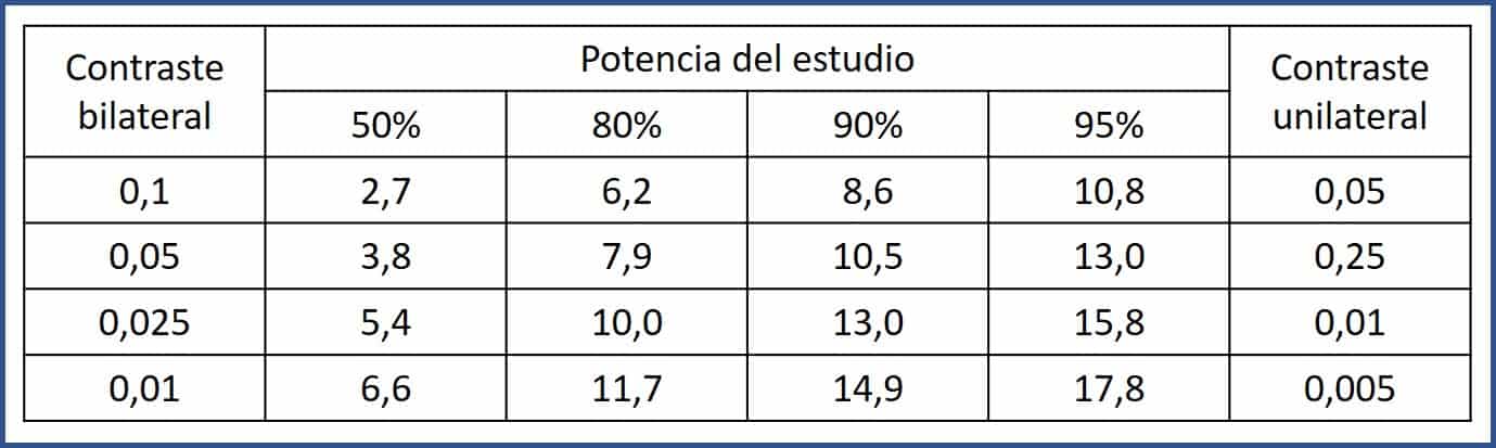
Where E is the number of events we need to observe, K is the value determined by the confidence level and the power of the study and lnRR is the natural logarithm of the risk rate.

The value of K is calculated as (Z_α + Z_β)², with z being the standardized value for the chosen confidence and power level. The most common is to perform a bilateral contrast (with two tails) with a confidence level of 0.05 and a power of 80%. In this case, the values ​​are Z_α = 1.96, Z_β = 0.84 and K = 7.9. In the attached table I leave you the most frequent values ​​of K, so you do not have to calculate them.

The risk rate is the ratio between the risk of the study group and the risk in the population, which we are supposed to know. It is defined as Sm₁ /Sm₂, where Sm₁ is the mean time of appearance of the event in the population and Sm₂ is the expected in the study group.

Let’s give an example to better understand what has been said so far.

Suppose that patients or treatment with a certain drug (which we will call A to not work ridiculously hard) are at risk of developing a stomach ulcer during the first year of treatment. Now we select a group and give them a treatment (B, this time) that acts as prophylaxis, in such a way that we hope that the event will take another year to occur. How many ulcers do we have to observe in a study with a confidence level of 0.05 and a power of 0.8 (80%)?

We know that K is worth 7.9. Sm₁ = 1 and Sm₂ = 2. We substitute their values ​​in the formula that we already know:

We will need to see 33 ulcers during follow-up. Now we can calculate how many patients we must include in the study (I find it difficult to enroll just ulcers).

Let’s assume that we can enroll 12 patients a year. If we want to observe 33 ulcers, the follow-up should last for 33/12 = 2.75, that is, 3 years. For more security, we would plan a slightly higher follow-up.

Survival curve comparison

This was the simplest problem. When we want to compare the two survival curves (we plan to do a log-rank test), the calculation of the sample size is a bit more complex, but not much. After all, we will already be comparing the survival probability curves of the two groups.

In these cases, the formula for calculating the number of necessary events is as follows:

We find a new parameter, C, which is the ratio of participants between one group and the other (1: 1, 1: 2, etc.).

But there is another difference with the previous assumption. In these cases, the RR is calculated as the quotient of the natural logarithms of π₁ and π₂, which are the proportions of participants from each group that present the event in a given period of time.

Following the previous example, suppose we know that the ulcer risk in those who are on A is 50% in the first 6 months and that of those who are on B, 20%. How many ulcers do we need to observe with the same level of confidence and the same power of the study?

Let’s substitute the values ​​in the previous formula:

We will need to observe 50 ulcers during the study. Now we need to know how many participants (not events) we need in each branch of the study. We can obtain it with the following formula:

If we substitute our values ​​in the equation, we obtain a value of 29.4, so we will need 30 patients in each branch of the study, 60 in all.

Coming to the end, let’s see what would happen if we want a different ratio of participants instead of the easiest, 1: 1. In that case, the calculation of n with the last formula must be adjusted taking into account this proportion, which is our known C:

Imagine we want a 2:1 ratio. We substitute the values ​​in the equation:

We would need 23 participants in one branch and 46, double, in the other, 69 in all.

We’re leaving…

And here we leave it for today. As always, everything we have said in this post is so that we can understand the fundamentals of calculating the necessary sample size in this type of study, but I advise you to use a statistical program or a calculator if you ever have to do it. There are many available and some are even totally free.

I hope that you understand now about Ezekiel’s message and that, in these studies, the things we do (or suffer) are more important than how many we do (or suffer). We have seen the simplest way to calculate the sample size of a survival study , although we could have bring unnecessary troubles into our lives and have calculated the sample size based on estimates of risks ratios or hazard ratios. But that is another story…