
Standardization.

Standardization is described, which consists of subtracting the mean from a value and dividing it by its standard deviation.
But I don’t accept any bar. It must be a very special bar. Or rather, a series of bars. And I’m not thinking about a bars chart, those so well-know and used that PowerPoint makes them almost without you asking for it. No, these graphs are very dull; they just represent how many times it repeats each of the values of a qualitative variable, but tell us nothing more.
Histogram and probability density
I’m thinking about a much meaningful plot. I’m thinking about a histogram. Wow, you’ll say, but isn’t it another kind of bar chart?. Yes, but it has a different kind of bars, much more informative. To begin with, the histogram is used (or it should be) to represent frequencies of continuous quantitative variables. The histogram is not just a bar graph, but a frequency distribution. What does that mean?.
Well, at the bottom, the bars are somewhat artificial. Let’s suppose a continuous quantitative variable such as weight. Imagine that our distribution ranges from 38 to 118 kg of weight. In theory, we can have infinite weight values (as with any continuous variable), but to represent the distribution we divide the range into an arbitrary number of intervals and draw a bar for each interval so that the height of the bar (and therefore its surface) is proportional to the number of cases inside the interval. This is a histogram: a frequency distribution.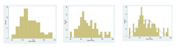
Now, suppose we make the intervals more and more narrow. The profile formed by the bars is increasingly looking like a curve as intervals narrow. In the end, what we’ll come up with is a curve, which will be called the probability density curve. The probability of a given value will be zero (one would think that it should be the height of the curve at that point, but it is not other than zero), but the probability of the values of a give interval is equivalent to the surface area under the curve in that interval. And what will be the area under the entire curve?.
Very easy: the probability of finding any of the possible values, i.e., one (100% if you like percentages).
As you see, the histogram is much more than what it seems at first sight. It tells us that the probability of finding a value lower than the mean is 0.5, but not only that, because we can calculate the probability density of any value using a tiny formula that I prefer not to show you to avoid you closing your browsers and stopping reading this post. Moreover, there’s a simpler way to find it out.
With variables following a normal distribution (the famous bell) the solution is simple. We know that a normal distribution is perfectly characterized by its mean and standard deviation. The problem is that each normal curve has its own distribution, so the probability density curve is specific to each distribution. What can we do?. We can invent a standard normal distribution whose mean is zero and whose standard deviation is one and we can study its probability density so that we need neither formulas nor tables to know the probability of a given segment.
Standardization
Once done, we take any value of our distribution and transform it into its soul mate in the standard distribution. This process is called standardization and is as simple as subtracting the mean from the value and dividing the result by the standard deviation. Thus we obtain another statistic that physicians in general, and particularly statisticians, venerate the most: the z score.
The probability density of the standard distribution is well known. A z-value of zero is in the mean. The range of z = 0 ± 1.64 comprises 90% of the distribution; the rage of z = 0 ± 1.96 includes 95%; and z = 0 ± 2.58, 99%. What we do in practice is to choose the desirable standardized z value for our variable. This value is typically set at ±1 or ±2, according to the variable measured. Moreover, we can compare how the z-score is modified in successive determinations.
The problem arises because in medicine there’re many variables whose distribution is skewed and does not fit a normal curve, such as the height, blood cholesterol, and many others. But do not despair, mathematicians have invented a stuff called the central limit theorem, which says that if the sample size is large enough we can standardize any distribution and work with it as it fit the standard normal distribution. This theorem is a great thing because it allows standardizing even non-continuous variables that fit other distributions like the binomial, Poisson, or other.
We’re leaving…
But all this does not ends here. Standardization is the basis for calculating other features of the distribution such as the asymmetry index and kurtosis, and it is also the basis for many hypothesis contrasts seeking a known distribution to calculate statistical significance. But that’s another story…