Chi-square test for independence.

Chi-square test for independence compares the proportions of two qualitative variables to determine whether or not they are independent.
I guess this phrase doesn’t have any meaning to the youngest of you or, at best, it will make you laugh as old fashioned. But I’m sure it brings back good memories to those of the same age than me, or older. The good old days when you started a conversation with this phrase, knowing you cared very little what the answer was, provided you didn’t be sent to hell. That could be the beginning of a beautiful friendship… and even more.
So as it happens that me, for better or for worse, ages have passed since the last time I said it, I’m going to invent one of my nonsense stories to have the excuse to re-use it and, incidentally, tire you out with the benefits of the chi square test. You’ll see how.
Let’s see an example
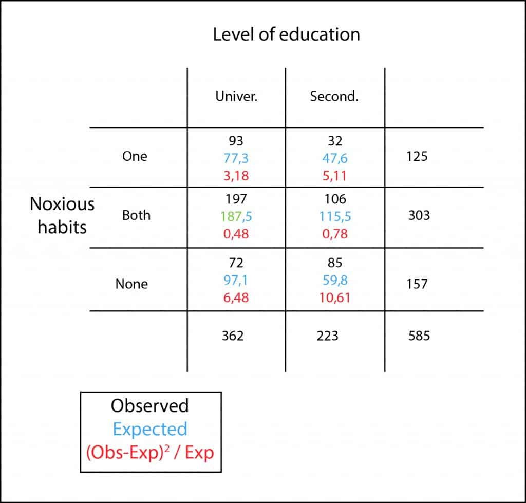
Let’s suppose that, for some reason, I want to know if the education level has any influence in having habits like smoking or drinking alcohol. So I select a random sample of 585 21-year-old women and ask them, and that’s the best: studying or working?. Thereby I classified them by education level (university and high school) and, thereafter, I check if they have one of the two habits, both or none of them. Finally, with these results I build my proverbial contingency table.
We can see that, in our sample, college students have higher rates of smoking and alcohol intake. Only 19% (72 out of 362) do neither the one nor the other. This proportion rises to 38% (85 out of 223) among high school students. Therefore, consumption of tobacco and alcohol is more prevalent among the former but, can this result be extrapolated to the global population or can the observed differences be due to chance by random sampling error?. To answer this question is what we needed our chi square test for.
Chi-square test for independence
First, we calculate the expected values multiplying the marginal value of each cell’s row by the marginal of its column, and divide the result by the table’s total. For example, to calculate the expected value in the first cell would be (125×362) / 585 = 77.3. So, we do the same for all cells.
Once we have calculated all the expected values, what we want to know is how far away they are from the observed ones and whether this difference can be explained by chance. Of course, if we add the calculated differences, positives and negatives ones will cancel each other and the total result will be zero. This is why we use the same trick that is used to get the standard deviation: we squared the differences before adding them, disappearing negatives values as a result.
Moreover, any given difference can be more or less relevant according to its expected value. The error is greater is we expect one and get three than if we expect 25 and get 27, although difference equals two in both cases. To offset this effect we can standardize this difference dividing it by its expected value.
And now we add all these values and come up with the total sum of all cells obtaining, in our example, a value of 26.64. We just need to explain the question of whether 26.64 is too large or too small to be explained by chance.
We know that this value approximately follows a chi square frequency distribution with a number of degrees of freedom equals to (rows-1) plus (column-1), which are two in our example. So we just have to calculate the probability of that value or, what is the same, its p.
This time I’m going to do it with R, the statistical software you can find on and download from the Internet. The command for doing it is the following:
pchisq(c(26.64), df=2, lower.tail=FALSE)
We obtain a p value less than 0.001. As p < 0.05 we can reject our null hypothesis that, as usual, states that the two variables (education level and bad habits) are independent and the observed differences are due to chance.
Conclusion
So what does this mean?. Well, it simply means that the two variables are not independent. But no one would ever think that this result implies causality between the variables. This does not mean that studying more make you smoke or drink alcohol, but simply that the observed distribution between both variables is different from what would be expected by chance alone. This may be due to these variables or to other that we haven’t even considered. For instance, it strikes me that age in both groups might be a more logical explanation of that situation that, on the other hand, is just a product of my imagination.
We’re leaving…
And once we know the two variables are dependent, will the strength of this dependence be stronger the higher the chi or the lower the p?. Certainly not!. The higher the chi or the lower the p, the lower the probability of being wrong and commit a type 1 error. If we want to know the strength of the association we have to rely in other parameters such us risk ratio or odds ratio. But that’s another story…
