Step by Step. Student’s t test for independent samples.

Student’s t test allows comparing two independent means with small samples and without knowing the population variance.
We saw in a previous post how William Sealy Gosset, with the help of some friends, designed a probability distribution in order to carry out his noble endeavor to improve the production of Guinness distilleries.
This distribution was published under a pseudonym, which is why it is known as Student’s t distribution, instead of Gosset’s t, or something similar.
Student’s t probability distribution allows to compare two means when the samples are small and the population variance is unknown, a situation that is quite frequent.
So, using a story that is the fruit of my imagination (although it could well be true), let’s see how Gosset took advantage of this new distribution.
Some preliminary preparations
Let’s suppose that a given fertilizer has been used so far on the distillery’s farm, which we will call A so as not to try too hard, but that someone have been doing some experiments with a new one, which we will call B.
Fertilizer B does increase malt production, but Gosset believes that beer made with this malt is slightly more acidic, which, if true, would rule it out as a substitute for classic fertilizer A.
To clear up any doubts, Gosset decides to divide a section of the farm’s land into 50 different plots, sowing each one of them and using, at random, fertilizer A in 25 of the plots and B in the other 25 ones.
Once the cultures are obtained, he brews the beer and measures the pH of each of the 50 samples. The result obtained can be downloaded from this link.
Now that we have the data, let’s see if the Gosset impression is correct.
Step 1. Descriptive analysis of the data
We launch the R program and open RCommander with the command library(Rcmdr). We select the menu option Data-> Load data set… and load the file that we obtained with the link that I provided above. If you look at the active dataset, its name is “cultivos” (if not, select it).
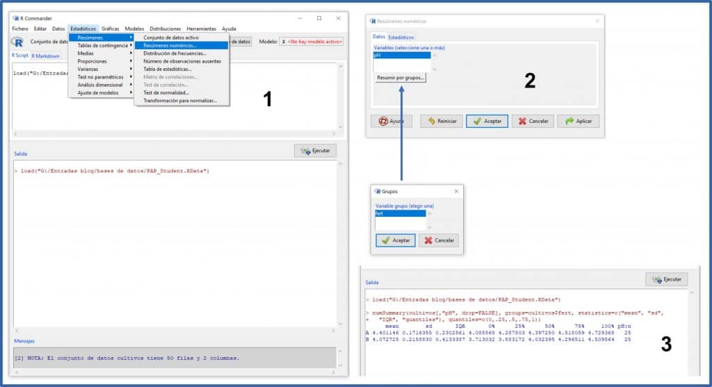
Since we have the data loaded, let’s see what the pHs of the two samples are. We select the menu Statistics-> Summaries-> Numerical Summaries. In the pop-up window we select the variable “pH” (the only quantitative one is this data set) and click on the button “Summarize by groups …” to select the variable “fert” (the type of fertilizer).
If we did not make the selection by groups, R would show us the analysis of the 50 samples as a whole, but we are interested in seeing the pH of the samples of the two fertilizers separately. You can see all this in figure.
If you look at the output window (3), R provides the sample size, the mean, the standard deviation, the interquartile range (IQR), the maximum and minimum values (100% and 0%), the median ( 50%) and quartiles (25% and 75%).
In effect, the mean pH of group A is 4.40 and that of group B 4.07. It seems that, indeed, the beer obtained with fertilizer B is more acidic, at least in our sample. However, this difference may be due to chance, since we are using a small sample and there is some dispersion of the data (0.17 and 0.21 pH units in groups A and B, respectively).
It is possible that if we repeated the experiment, the result would be different.
Well, to measure the probability that the difference we observe is due to chance, we will use the Student’s t test.
Step 2. Checking normality of data
Student’s t test compares the means of a continuous variable classified according to the two categories of a dichotomous nominal variable. These two groups can be independent (each subject can only belong to one of the two categories) or be paired samples.
In our case, we will use the Student’s t test for independent samples, once we verify that two assumptions are met:
- The continuous variable follows a normal distribution for the two categories of the nominal variable.
- There is homoscedasticity, which means that the variance of the values of the continuous variable is the same in the two groups of the dichotomous nominal variable.
Let’s first check if the assumption of normality is fulfilled.
We select the menu Statistics-> Summaries-> Test of normality… In the pop-up window we select the variable “pH” (the only quantitative there is is this data set), we mark the test that we want (for example, Shapiro-Wilk) and click on the button “Test by groups …” to select the variable “fert” (the type of fertilizer). Finally, we click on accept button and we obtain the result in the output window (next figure).
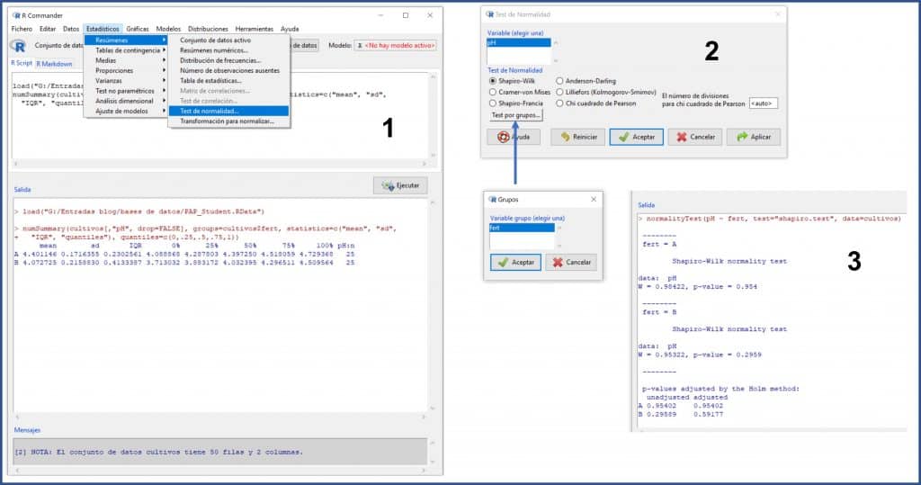
The values of the W statistic for fertilizers A and B are 0.98 and 0.95, respectively, with a statistical significance value of p = 0.95 for group A and p = 0.29 for group B. As p> 0.05 in both groups, we cannot reject the null hypothesis that, for the Shapiro-Wilk test, assumes that the data follow a normal distribution.
However, we already know that numerical tests to check normality are not very powerful, especially if the sample is small, so it is advisable to check their result with some graphic method.
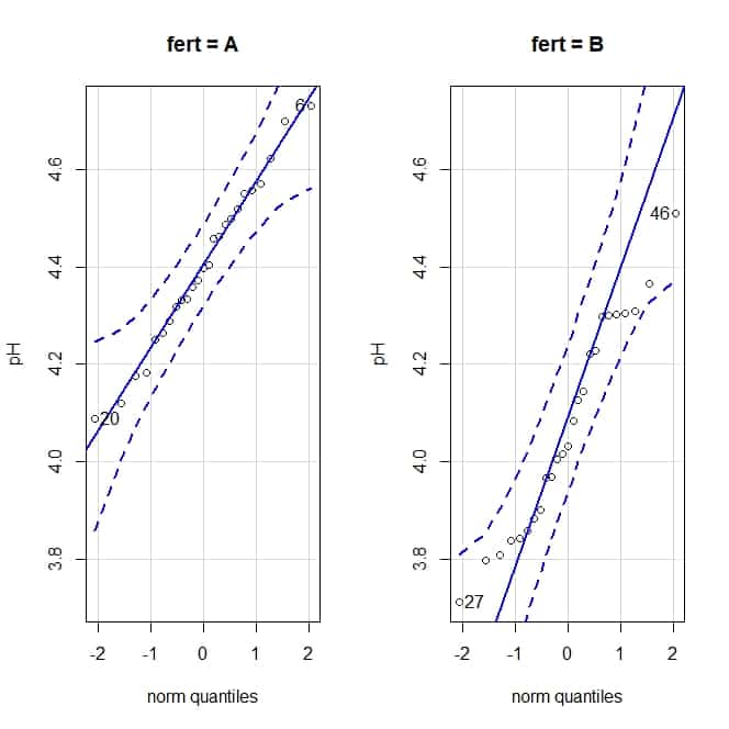
We are going to draw the quantile comparison graphs. To obtain them, we select the menu Graphs-> Quantile comparison graph… and, in the pop-up window, we click the button “Graph by groups” to obtain the graphs for each fertilizer, which you can see in the attached figure.
The quantile comparison graphs compare the values of the quantiles of the distribution with what they should be if the data followed a normal distribution. If this is the case, the values are aligned along the diagonal of the graph. Looking at the graphs, we can assume the normality of our data (although there is some deviation in the case of group B values).
Step 3. Checking homoscedasticity
We know that the quotient of two variances follows a Snedecor’s F probability distribution.
In the case of homoscedasticity, the value of this quotient must be close to unity. The further it moves away from unity, the greater the probability that the variances are actually different and that the observed difference is not due to chance.
To calculate this probability, we can perform the Snedecor’s F test, which takes into account the degrees of freedom of the numerator and denominator of the quotient of variances.
We select the menu Statistics-> Variances-> Test F for two variances… In this simple case, we just have to press “OK” in the pop-up window and R will show us the results in the output window, as you can see in the next figure.
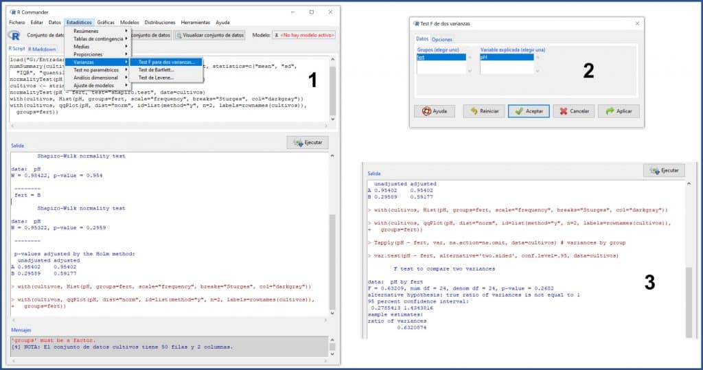
We can see in various ways that the homoscedasticity assumption does indeed hold.
First, the value of the statistic F = 0.63, with a p = 0.26, so we cannot reject the null hypothesis that, for this test, assumes that the two variances are equal.
Also, if you look at the final part of the results, the ratio of variances is 0.63, with a 95% confidence interval of 0.27 to 1.43. Since the interval includes the null value (the unit), we can say that the observed difference between the two variances is not statistically significant.
Step 4. Let’s do a Student’s t test
Now we only have to carry out the hypothesis testing, using the Student’s t test for independent samples. In this contrast, the null hypothesis of equality of means is assumed (the observed difference is due to chance).
We select the menu Statistics-> Means-> Test t for independent samples… (as you can see in the next figure). A window will appear (2), in which the variables are already selected, and we will click on the “Options” tab (3) to mark that we want a bilateral contrast and that we assume the equality of variances. We accept everything and R gives us the result in the output window.
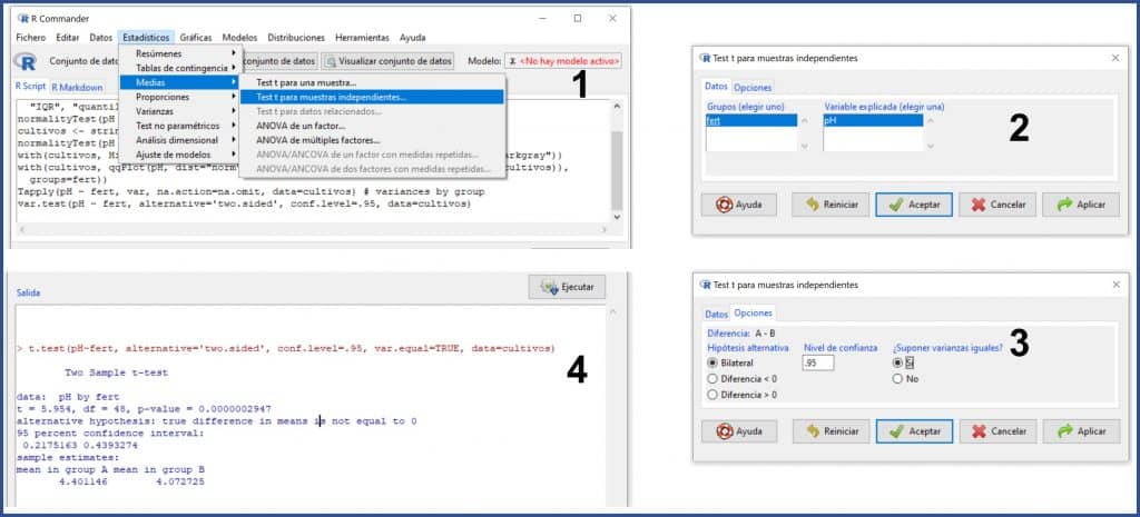
We can see that t = 5.95, with a p value much lower than 0.05, with which we can rule out the null hypothesis of equality of means and assume that the observed differences are due to the fertilizer used. In other words: Gosset was right and fertilizer B makes for a more acidic beer.
We’re leaving…
In this post we have seen how to compare two independent means when the sample is small, provided that the assumptions of normality and homoscedasticity are met. But what can we do if these assumptions are not met? In these cases we have three options.
The first is to use the Student’s t test if the sample is large and the deviation is slight. If the sample is not very small, Student’s t is quite robust in the event of non-compliance with these assumptions, especially that of normality.
Second, we can try to transform the data and see if the transformed data does follow the normal distribution.
The third option, perhaps the most advisable, is to use the non-parametric equivalent of the Student’s t test, which is none other than the Mann-Whitney U test. But that is another story…

