MICE: advanced data imputation.

In 2014, a group of mice became pioneers in a historic mission: Rodent Research-1, NASA’s first official experiment to send rodents to the International Space Station. It was quite a scientific milestone… though the mice probably weren’t as thrilled. While the astronauts orbited Earth at 28,000 km/h, the dutiful rodents floated around in microgravity, generating valuable data on how space affects mammals. But of course, since none of the mice held a press conference upon their return, a lot of details were left hanging. So, once again, science had to fill in the blanks.

And that urge to complete what’s missing isn’t just a quirk of orbiting labs. For those who work with data, missing values are the daily bread of every analysis. Incomplete surveys, faulty sensors, misloaded records… If we don’t want our models to fall apart like a space station with loose bolts, we’ve got to find smart ways to complete the story without just making stuff up.

That’s where the true art of filling in with style comes in. And when I say “with style,” I’m not talking about pastel colors or fancy fonts, but about applying techniques that have solid foundations, are robust, and combine statistical elegance with practical smarts.

One of the most widely used and powerful techniques is Multiple Imputation by Chained Equations (MICE). The name might sound intimidating, but its logic is as elegant as it is precise. In this post, we’ll uncover the most surprising and counterintuitive secrets of the MICE algorithm, so you can use it confidently and accurately, without falling into statistical traps.

Not all missing data are created equal

Before applying any technique, we need to think about why the data are missing in the first place. Not all missing values are created equal, and MICE takes that very seriously. Depending on their origin, we can break them down into three main categories.

When data go missing completely at random, we call them (brace yourself) Missing Completely At Random (MCAR). This means that the probability of a certain variable having missing values doesn’t depend on any other variable in the dataset.

The second category is Missing At Random (MAR), similar to the first, but without the “completely.” Here, the probability of a variable having missing data depends on the value of another observed variable. Picture a survey where the “glycated_hemoglobin” field is mysteriously empty every time someone’s “blood_glucose” comes back normal (because only those with high glucose levels are asked for the hemoglobin). In that case, the missing hemoglobin values aren’t random—they depend on another variable: glucose.

The third type is Missing Not At Random (MNAR). This time, the absence is due to the value of the missing variable itself. Let’s say, just for fun, it’s a tax survey: folks with really high incomes might conveniently “forget” to report them.

The key point is that MICE works great for MCAR and especially MAR cases (which are the most common). But it’s not a good fit for MNAR data. So, knowing the nature of your missing data is crucial if you want to avoid using the wrong technique and ending up with biased results.

As we’ll see next, the reason MICE shines with MAR data lies in how it works: unlike simpler methods, it doesn’t try to “guess” each missing piece in isolation; it actively learns from the relationships between variables that explain why the data went missing in the first place.

MICE: an intimidating name for a simple logic

We’ve already mentioned that “Multiple Imputation by Chained Equations” might sound a bit overwhelming and excessively technical, but the truth is, the idea behind this algorithm is surprisingly intuitive. At its core, MICE doesn’t try to fill in all the blanks in one go. Instead, it follows an iterative process that gradually refines its estimates over time.

Here’s how it works: in each cycle, the algorithm picks a column with missing values, treats it as the “target variable,” and uses all the other columns as “predictor variables.”

Then, it trains a predictive model that learns the relationship between the predictors and the known values of the target variable. Once the model is trained, it’s used to predict the missing values in that column.

This whole routine is repeated for every column with missing data, and the process loops through the full dataset again and again until the values settle down and stop changing.

This chained approach is the secret sauce of the algorithm. Rather than treating each column in isolation, MICE takes advantage of the interconnections between variables. That’s why people say it “learns” from the rest of the data what’s missing in each variable.

So yes, the name might sound like something out of a sci-fi experiment involving overly intelligent rodents, but the underlying logic is more like a clever maze than a trap.

A practical example

To get a better feel for how the MICE method works for imputing missing data, let’s walk through a simple example with a small dataset I’m going to make up on the fly.

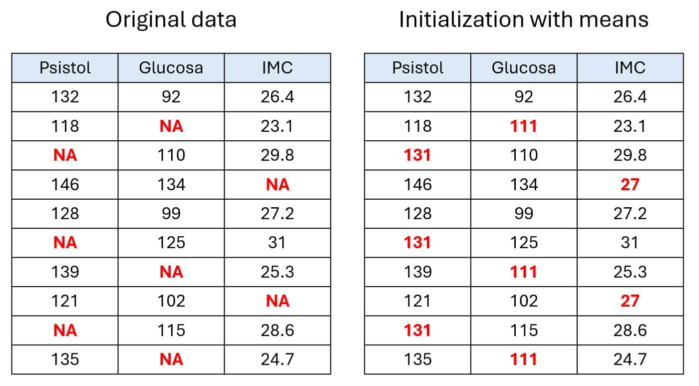
Let’s say we’ve collected data from 10 people, specifically their systolic blood pressure, blood glucose levels, and body mass index (BMI), as shown in the first table in the figure below.

As you can see, not all records are complete. Some cells are marked as NA, which is how the R programming language labels missing data. For this example, let’s assume the missing values are MCAR and MAR, the kinds MICE handles best.

The first step is a basic univariate initialization. That means we fill in all missing values with a simple estimate, like the mean of each column, since we’re dealing with quantitative variables. This gives us a full dataset, but it’s just a starting point, not the final imputed data. This initial version is what the algorithm uses to kick off the real work of refinement. You can see this in the second table.

❮

❯

Now comes the predictive refinement. The algorithm tackles each column with missing values one by one, in iterative cycles. In each step, it pulls out the NAs from the selected column and treats that column as the target variable, using the other columns as predictors.

Using this combo of data, it trains a predictive model to estimate the missing values of the target column. In my example, I used the mice package in R with predictive mean matching, which is similar to linear regression but considers the observed values too, so you don’t end up with impossible or weird estimates.

Once that column is filled in, those new values are used to predict the missing values in the next column, and so on.

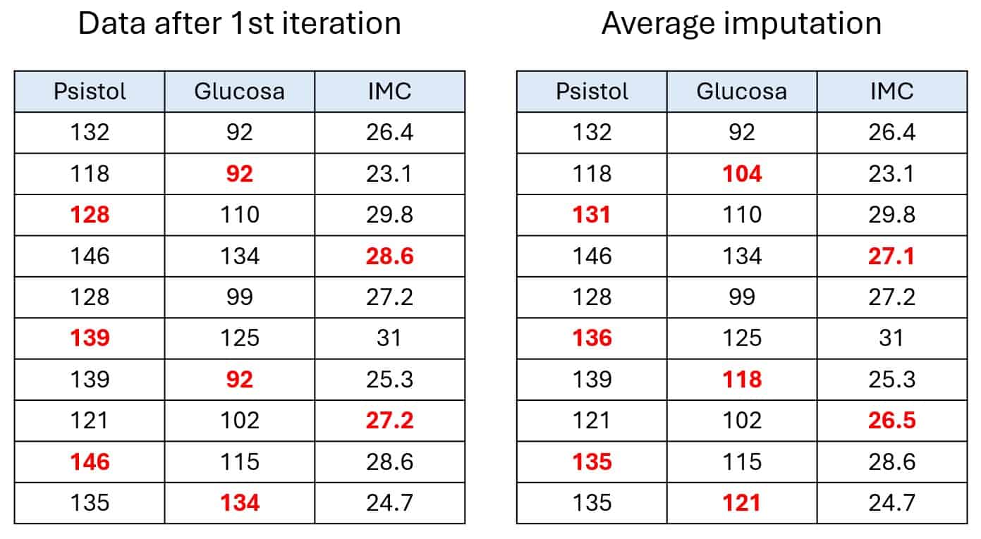
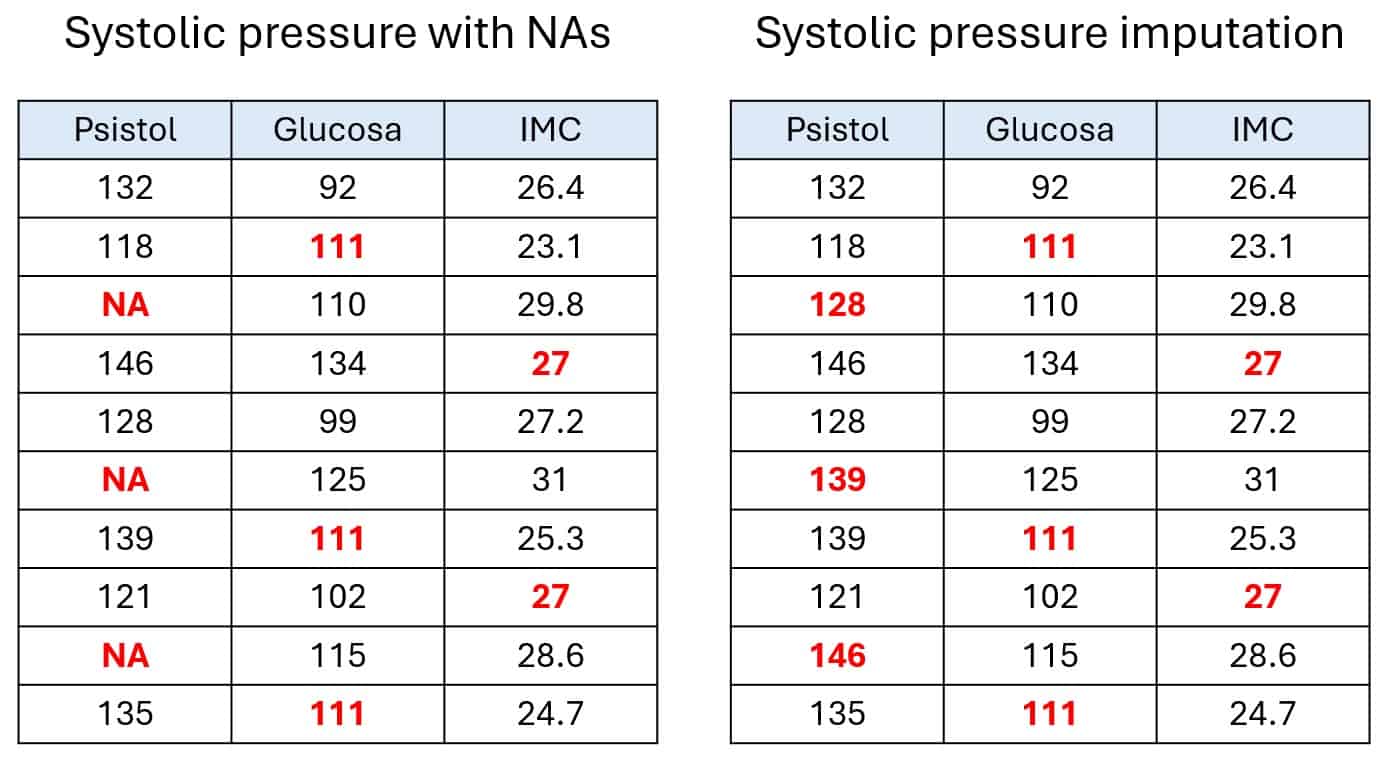
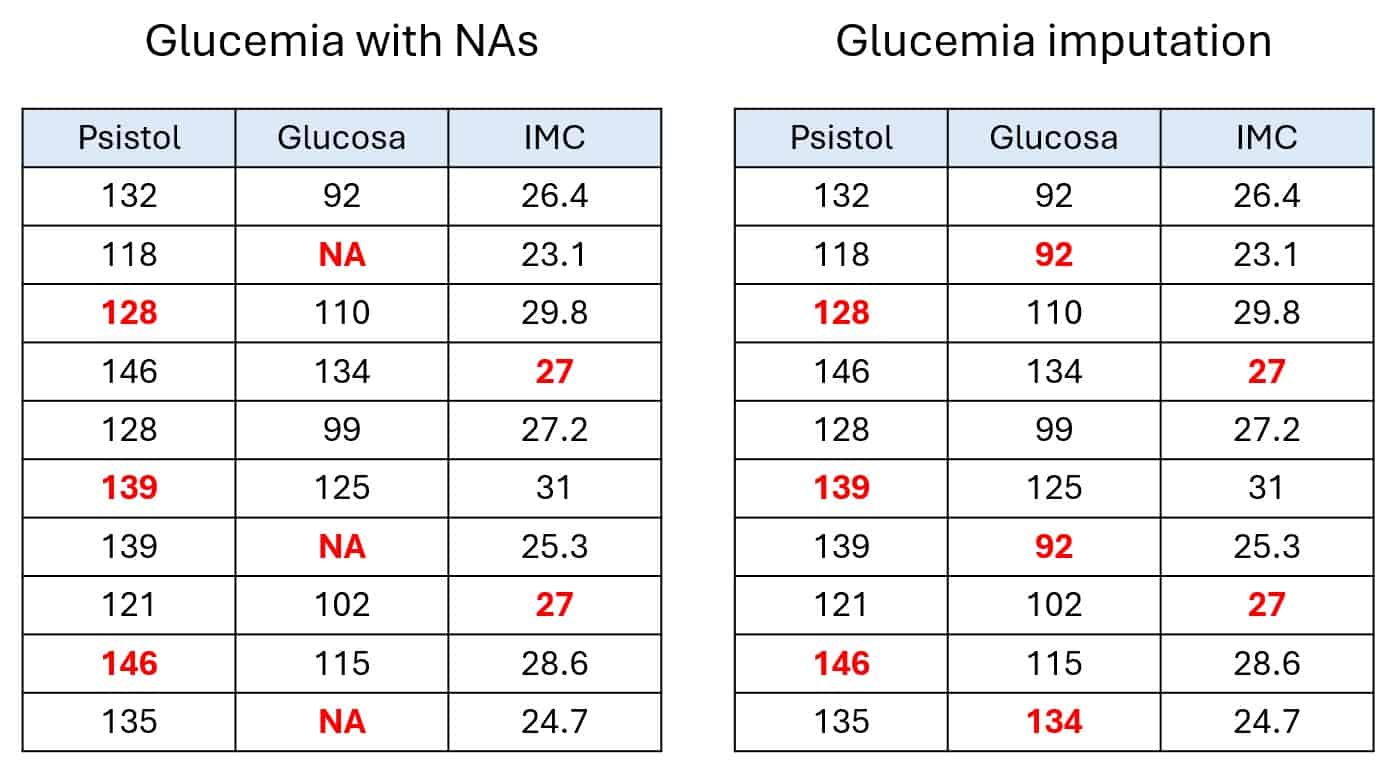
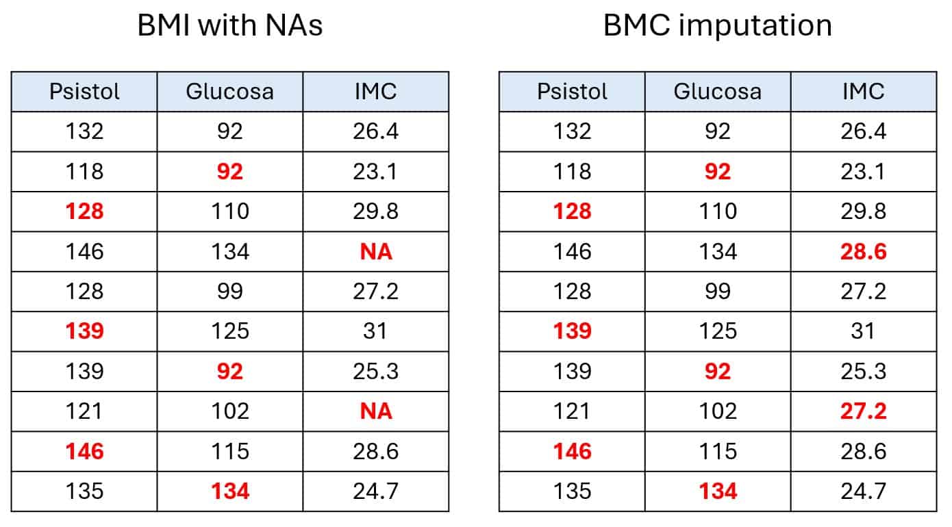
In the last pair of tables, you can follow the process through three cycles: blood pressure, glucose, and BMI. This whole thing repeats for a set number of cycles, generating several datasets per cycle. That gives us a final results table, as shown in the last two tables. (Okay, that part’s a bit of poetic license for teaching purposes; in real life, the model uses all the data in a more complex way, but let’s keep it simple.)

In case you're curious, I ran this example using 10 iterations with 5 datasets per iteration.

Filling in with style

Now we can appreciate the real power of MICE. The algorithm doesn’t just calculate a simple mean or median to plug the gaps: it treats imputation as a prediction problem. Think of MICE as a detective investigating a missing value. It doesn’t settle for checking the last known location (like the column’s mean); it interviews all the witnesses (the other columns) to build a predictive profile (a regression model or similar) of where that value should be.

This predictive, multivariate approach is exactly what makes MICE so effective for MAR data. It cleverly uses the other variables as clues to solve the missing-value mystery. Under the hood, MICE can even use advanced machine learning models like random forests or gradient boosting (XGBoost) to capture complex, non-linear relationships between variables and make more robust predictions.

Once again: more isn’t always better

Since it’s an iterative algorithm, it’s easy to assume that more repetitions will lead to better results. But that’s not necessarily true. In practice, it turns out the average of the imputed values tends to converge very quickly. In many cases, the values stabilize after just 4 or 5 iterations.

That’s something crucial for anyone working with data to keep in mind: even if it’s tempting to set a high number of iterations “just in case,” the reality is that it doesn’t buy you much, only wasted computing cycles. In other words: time and money, both of which are in short supply. The real skill lies in identifying the convergence point, which allows you to process even massive datasets efficiently.

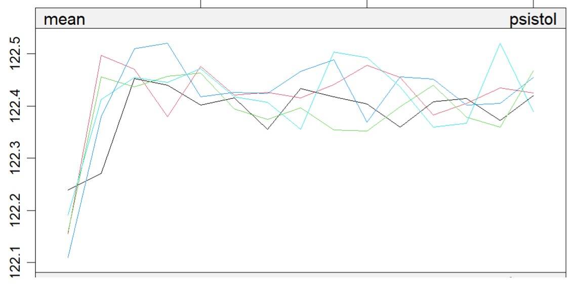
To help us figure out how many iterations are truly needed to reach convergence, we can plot the evolution of the mean values across successive imputations, just like the figure shown here. I’ll admit, though: I pulled a tiny trick. That chart was generated using a much larger dataset, just to make the pattern clearer.

Success speaks in silence

Now that we know how to run MICE efficiently by identifying its point of convergence, how can we tell if the final result is actually good? The answer doesn’t lie in the individual imputed values, but in their collective impact on the original character of the data.

The goal is to fill in the blanks without changing the “personality” of the variables. It’s like adding missing puzzle pieces without altering the overall picture.

A subjective but intuitive way to check quality is to compare the distributions of the variables (using histograms or density plots) before and after imputation. If the general shape of the distribution holds up, that’s a good sign. On the other hand, if the distribution changes dramatically (a different mode, fatter tails, unexpected skewness) then the imputation might be introducing bias that could mess with any machine learning model you train later on.

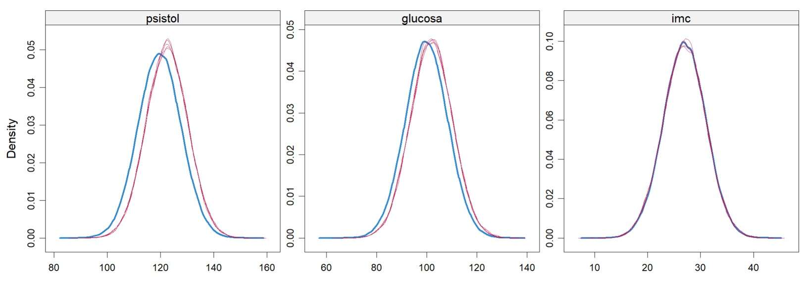
In the final figure, I show you the distribution of the complete data (thicker blue line) along with those from the imputations. As you can see, they’re pretty similar, so we can be happy with our results.

We’re leaving…

It seems that in the end, the mice weren’t just great astronauts; they also inspired us to find our way through a maze of missing values. MICE, that intimidatingly named method, reminds us that the goal isn’t simply to plug gaps, but to use the power of predictive models to make smart estimates based on the hidden relationships already buried in your data.

It’s this ability to detect those hidden patterns that explains why it works better with data that are missing at random, when the absence is tied to other variables in the dataset.

MICE is, in short, an elegant way to bring order to chaos: a system that learns from the data itself to fill in the blanks without betraying its original structure. Understanding that not all gaps are created equal, that its logic is predictive, and that convergence happens quietly, when the means stop shifting and the distributions stay steady, lets us use it with confidence. Imputing isn’t guesswork: it’s prediction with style.

We’ve already touched on the importance of picking the right number of iterations, since, as with any iterative algorithm, MICE can get a little overexcited and start learning noise instead of structure, the classic sin of overfitting, now in imputer form. But that’s not a hopeless fate: we have ways to keep our models from falling in love with their own data. But that’s another story…