Analysis of results in a crossover clinical trial

The analysis of a crossover clinical trial differs from that of a classical parallel trial. It must take into account the period and sequence effects.

Saving is an important determinant when conducting any study, especially if it is a usually costly and time-consuming clinical trial. So, researchers have tried to design new ways of doing studies that allow them to save time and money, most in regards to the number of participants needed, one of the main determinants of the final cost of the study.

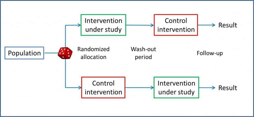
One such design is the crossover trial, which we discussed in a previous post. In this type of trial, each subject is randomized to a group, the intervention is made, there’s a washout period and the other procedure is performed as outlined in the figure you can see attached.

As each subject acts as his own control, the effect of confounding variables that may exist is limited; besides, there’s less variability than in studies in which intervention and control group’s people are different. This allows having a smaller sample size than in conventional parallel clinical trials.

To make a crossover trial, the effect must be rapid and of short duration, while remaining stable throughout the study periods. Otherwise we can find two methodological weaknesses of the crossover trial: the sequence effect and the period effect.

Periods of crossover clinical trials

Therefore, in addition to analyze the final effects of the two arms under study, we extend the statistical analysis of the data to be sure that wires are not crossed and we take for good a difference in effect size that, in fact, may be due to a methodological flaw of this type of trial.

This analysis is a bit laborious, so we are going to work with a completely fictitious example.

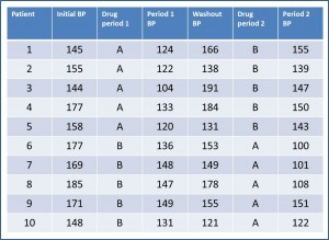
Let’s suppose we want to test two hypotensive drugs that we’re going to call A and B to not rack our brains too much. We’re going to do the example with 10 patients for simplicity’s sake, but imagine that there’re many more. In the first table we see represented the main results of the trial.

We have collected systolic blood pressure (BP) before starting the study, at the end of each period and at the end of the washout period of the test. Of course, we collect also what drug has received each participant during each period.

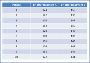
The first thing we think of is to compare the differences in BP between the two drugs. For that we need to extract the data and rearrange them. With them we build the second table. If you take the trouble to calculate them, the mean (m) of BP after receiving A is 118.5 mmHg, with a standard deviation (s) of 16 mmHg.

Corresponding values for B are m = 144.5 and s = 7.24. To determine whether these differences are significant we do a hypothesis test, setting the null hypothesis (H0) of no difference in effect. Let us assume that the variable is normally distributed, the variances are equal and that the sample was much larger in order to use the Student’s t test for paired data.

If you calculate the value of t with 9 degrees of freedom, it is equal to -5.18, which corresponds with a value of p = 0.0005. As p <0.05 we reject the null hypothesis and conclude that drug A produces a greater reduction in BP that drug B.

And here the analysis would end if we were analyzing a parallel trial, but in our case we’ve to do some more checking to be sure that we don’t get our wires crossed because of the methodological weaknesses of the crossover trial.

Analysis of results

First, we’ll check that the effect of the interventions is short and there is no residual effect of the first intervention when the second begins. If there is no residual effect, the BP at the end of the washout period should be similar to the basal BP, before any intervention.

The basal BP has a m = 162.9 mmHg, with s = 14.81. For its part, the values at the end of the washout period are 156.6 and 23.14 mmHg, respectively. If we do the corresponding contrast, the value of t is 0.81, with p = 0.43. We cannot reject the H0 of equality, so we conclude that the BP is similar before the first intervention and at the end of the washout period, and then there is no residual effect.

Second, we’ll check that there is not a period effect. If this occurs, the effect at the end of the second period would be higher (or lower) than at the end of the first. At the end of the first period we find a BP’s m = 131.4 mmHg with s = 14.44 mmHg. At the end of the second values are 131.6 and 21.77 mmHg, respectively. By making the contrast we find a value of t = -0.02, p = 0.98. Conclusion: we don’t reject the H0 of equality and conclude that there is no evidence of an effect period on the trial.

Finally, we will investigate whether there might be a sequence effect. If this exists (there’s an interaction between the two interventions), the effect of each of the interventions could be different depending on the order in we performed each of them. For this we’ll calculate the median decrease in BP in all patients when using AB sequence and compare it with that found using the BA sequence.

For AB sequence, data are m = -26.2 mmHg and s = 11 mmHg.  For BA sequence is -25.8 and 21.22 mmHg, respectively. The value of the Student’s t test is -0.04, which corresponds to a value of p = 0.96. Again, we cannot reject the H0 of equality and conclude that there is no a sequence effect.

We’re leaving…

And with this the analysis is done. The final conclusion is that there is a statistically significant difference in hypotensive potency of the two drugs in favor of A, and that we found no signs suggesting residual effects of an intervention over another, neither a period nor a sequence effect.

Remember that the data are fictitious and we have assumed normality and equality of variances for teaching purposes. Moreover, as we noted at the beginning, it would not be entirely correct to use the Student’s t test with such a small sample, but I took this little license to explain the example more simply. Anyway, having a computer’s program it costs the same effort to make a Student’s t test than a Wilcoxon’s.

And that’s it. You see, the statistical analysis of the results of a crossover trial is far more laborious than that of the parallel trial. Anyway, we have seen the simplest example, when there is no interaction between the two interventions. And that is so because when there is interaction analysis does not end here and further checks are necessary. But that is another story…