Fisher’s z.

In the world of numbers, there is a magical kingdom called Probabiland, where every corner is impregnated with the excitement of statistics and the magic of probabilities. Rivers flow with data, forests are filled with regression trees, and in the mountains, peaks reach heights proportional to their statistical significance.

One of the most popular places in the kingdom is the majestic Palace of Probabilities, a casino where each table is a statistical adventure, and each card reveals a secret hidden in the data. Players can explore the gaming tables, from regression roulette to hypothesis testing poker, to non-linear correlation blackjack or discrete distributions, for the more daring.

We are going to stop at the “Reduced Samples” table, where the cards are piled up in small piles of data and uncertainty reaches its highest levels. At this table we will see two common players, Pearson’s R and Fisher’s z.

Pearson’s R, known for its mathematical elegance, is like a reliable card that always adds up to 1. But, although it is ideal for secure, linear connections, it faces challenges in tiny samples, where imprecision can significantly impact its estimation ability, demanding extra caution in interpreting the results.

In contrast, Fisher’s z, with its touch of statistical intrigue, acts as the wild card that can change the game in an instant. It is capable, even though the sample is small, of maintaining its precision with a certain elegance.

Today we are going to stay in this corner of the statistical casino, where R and z come together to face the challenge of small samples, collaborating in meta-analyses in which the effect measure is a correlation, and the sample sizes of the primary studies are limited.

Pearson’s correlation coefficient

We already know that one of the objectives of a meta-analysis is to obtain a global outcome measure that summarizes the results of each of the studies included in the systematic review. This measure provides a general estimate of the effect of interest, combining information from all studies considered.

When the effect studied is a correlation, the parameter most frequently used is the product-moment correlation coefficient, better known as the Pearson’s correlation coefficient (R).

We can calculate R between two quantitative variables by dividing the covariance of the two variables by the product of their standard deviations, according to the following formula:

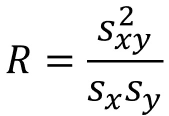
If we look a little at the formula, R is nothing more than the covariance standardized by the standard deviations, which makes it possible to compare different correlation coefficients without their values being affected by the measurement scales of the variables.

This is a point in favor of Pearson’s R, but we will see that it has other properties that are not so favorable, especially when we handle small sample sizes.

We know that the global measure that we calculate in a meta-analysis tries to be an estimate of that measure of correlation existing in the general population, which is unreachable. To make this estimate, we calculate a confidence interval, usually at 95%, which gives us an idea of the uncertainty and the margins between which the population measurement may be.

Well, the problem with Pearson’s R is that its variance depends greatly on the sample size of the data with which it was calculated. We can see its formula in the following formula:

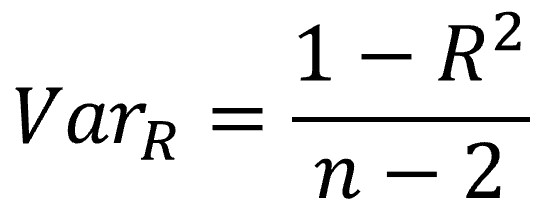
The first thing we see is that R is in the numerator subtracting from 1, so the numerator will be smaller as the value of R increases (so the variance will decrease). We see it in scatter diagrams if we represent two quantitative variables. When the correlation is greater, the variability of the data is lower, and the point cloud has a more elongated shape. When the correlation is lower, the cloud will be more circular, there will be more variability in the data.

The value of R does not depend on us but is a characteristic of the relationship between the two quantitative variables. But there is another component in the formula on which we can act: the sample size (n).

Since the sample size is in the denominator, the variance will increase as the sample size decreases. Look at the first figure, which represents the sample size on the abscissa and the variance on the ordinate. Let’s focus, for now, on the blue line, which represents the variance of Pearson’s R (later we will see what the red line means).

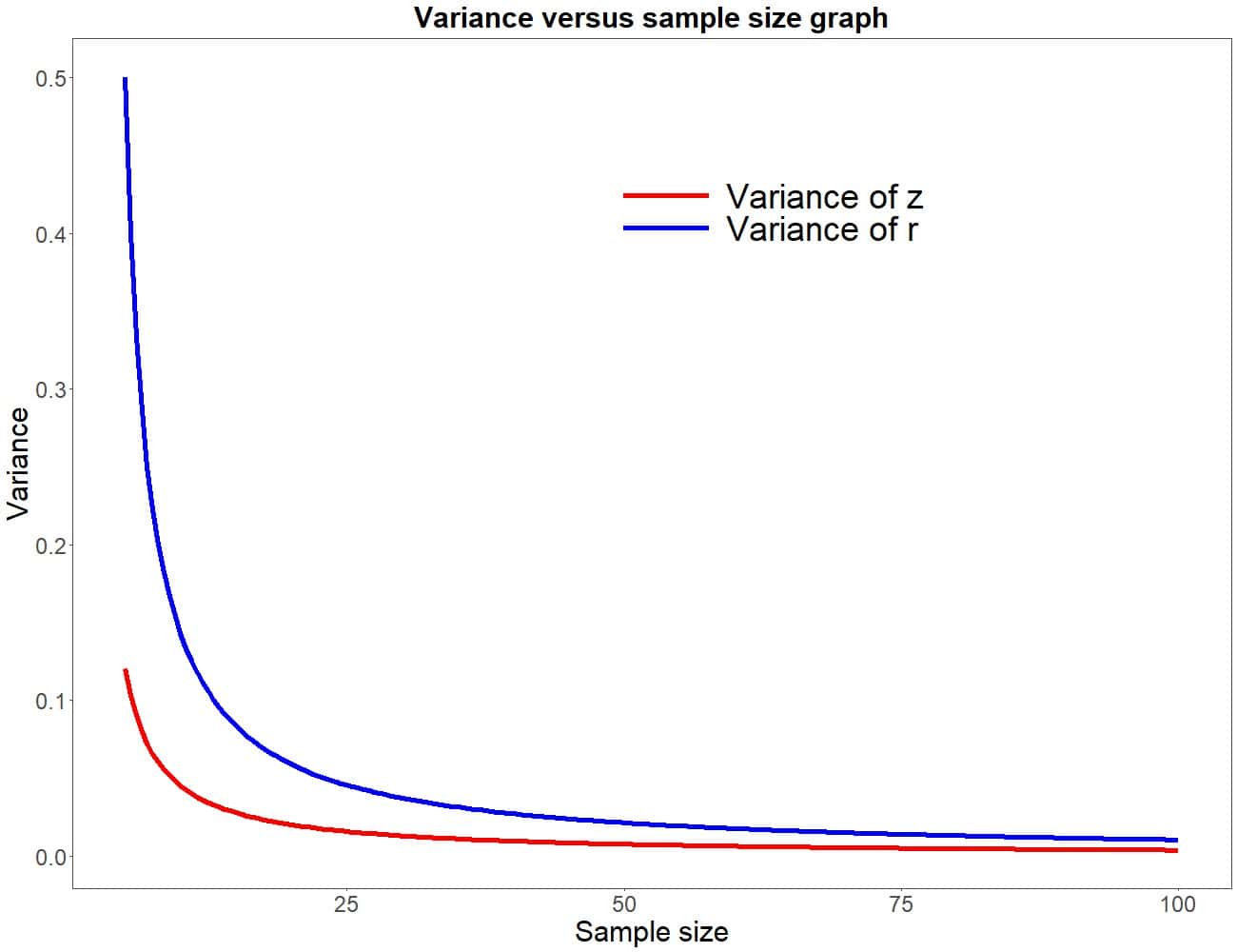
We can see how the variance begins to rise as n decreases, taking a very high slope with sizes less than 20 participants. In other words, the variance becomes almost exponentially larger (more unstable) with smaller sample sizes.

This has an unintended consequence. R estimates are based on the point estimate (the R value of each study) and the standard error (which is the square root of the variance), so they will be more imprecise when the sample size is small, a situation that is occurs relatively frequently when we deal with the primary studies of a meta-analysis.

As the sample size increases, the correlation coefficient estimates become more stable and closer to the true population correlation. However, in small samples, values may fluctuate more due to increased variability of estimates.

More simply put, and to emphasize its importance, sample size can have an impact on the interpretation and reliability of Pearson’s correlation coefficient estimates.

This is the reason why, in these situations, it is advisable to perform a transformation to obtain Fisher’s z (which is not equivalent to the z of the normal distribution and the z score), which performs better with smaller samples than Pearson’s R.

Let’s see what it consists of.

Fisher’s z

As we have already said, to calculate the global measure when the sample sizes are small, instead of directly using the correlation as a measure of effect, it is transformed using the inverse hyperbolic arctangent function, also known as the Fisher’s transformation.

Don’t be alarmed, behind these offensive words lies a fairly simple formula:

We will understand the usefulness of Fisher’s z if we look at the formula to calculate its variance:

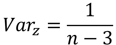
You will say that it still has the value of n in the denominator, like the variance of R, and that the variance is greater when the sample size decreases. This is true, but it is also logical that it happens. We already know that, in general, and for the same level of confidence, the precision of an estimate increases (its confidence interval will be narrower) when the sample size increases and/or variability decreases, and vice versa.

But look now at the red line in the previous graph that we previously decided to ignore. Represents the variance of Fisher’s z as a function of sample size. Although we see that the effect is like that suffered by Pearson’s R, its magnitude is much smaller, so z will be much more precise than R when the sample is small.

The reason behind this transformation is related to the statistical properties of probability distributions. It is like when we apply a logarithmic or inverse transformation such to a series of non-normal data to force the transformed data to be distributed normally and to be able to apply a test that assumes the normality of the data.

As transformed correlations behave closer to a normal distribution, statistical methods based on normality will work more appropriately. In particular, when performing a meta-analysis, the Fisher’s transformation allows the effect sizes of individual studies to be combined more accurately and appropriately, since many meta-analysis methods assume a normal distribution of effect sizes.

In any case, when we see a publication on one of these meta-analyses, we will probably not see the z anywhere and the authors will only show the Pearson’s correlation coefficient.

This has its reason. It is usual to use a statistical program to perform the meta-analysis. One of the options that we can tell the program is to perform this transformation. In that case, the Pearson’s coefficients of the primary studies will be transformed into their Fisher’s z equivalents, the program will perform all the calculations with Fisher’s z and, upon completion, it will perform the inverse transformation to present the reader with the Pearson’s coefficient. which is usually easier to interpret for most readers.

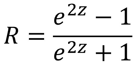
We can transform Fisher’s z into its R value by applying the following formula:

A practical example

The truth is that, in practice, we do not need to pay much attention to everything we have explained, since statistical programs take care of these details. In any case, it doesn’t hurt to know how and why things are done.

Let’s perform a simple example of meta-analysis with primary studies whose outcome variable is a correlation. To do this, we are going to use the R program (not to be confused with the R correlation coefficient) and a fictitious meta-analysis that we are going to invent on the fly to try to estimate the correlation that exists between the levels of magnetic fildulastrin and those of foolsterol in that terrible disease that is fildulastrosis.

If you feel like it, we can continue together step by step.

1. We load the necessary libraries in R:

library(tidyverse)

library(meta)

If you do not have these packages installed, it is necessary to install them before using them the first time using the install.packages() command.

2. Create our data set: We are going to create a data set with 15 completely made-up studies. To do a correlation meta-analysis with R we only need the value of Pearson’s R coefficient (not transformed) and the sample size of each study. We added it to the data set, along with a third column with the name of the study (capital letters A to O, to keep things simple). We create the three variables (vectors in R) and assemble them into a dataframe:

R <- c(0.58, 0.62, 0.54, 0.52, 0.76, 0.69, 0.66, 0.58, 0.62, 0.81,
0.49, 0.60, 0.79, 0.43, 0.69)
N <- c(18, 22, 45, 15, 20, 22, 24, 30, 50, 35, 14, 20, 16, 38, 40)
S <- LETTERS[1:15]
data <- tibble(S, N, R)

3. We do the meta-analysis: we are going to use the metacor() function from the R meta package. Although this function admits many parameters, we are going to make the model as simple as possible:

meta <- metacor(cor = R,
n = N,
sm = "zcor",
studlab = S,
data = data,
comb.fixed = FALSE,
comb.random = TRUE)

We have indicated to the program where the values of the untransformed Pearson correlation coefficients (cor), the sample sizes (n), and the names of the primary studies (studlab) are located, all within the indicated data set (data). Finally, we ask it to apply a random effects model, do the Fisher’s transformation (sm=”zcor”), and store the result in an object called meta.

4. We obtain the results: to do this, we simply execute the summary(meta) command.

In the second figure you can see the results output that the program offers us.

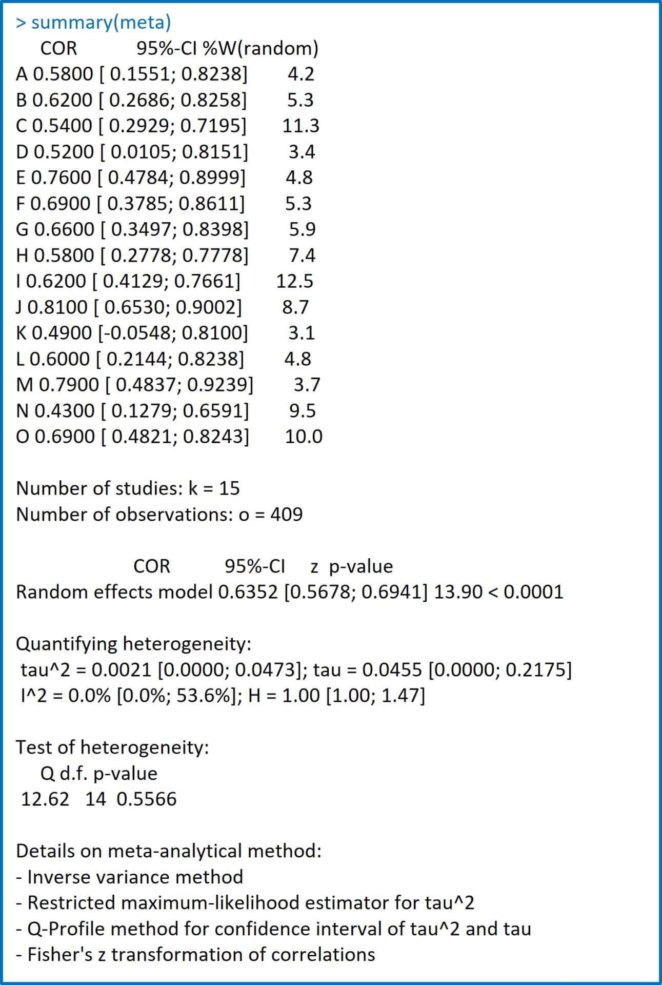
Firstly, it shows us a table with three columns with the list of studies with their Pearson’s coefficients (the ones we introduced), the 95% confidence intervals that it estimates for each of them and the weighting that it establishes for each study. for the calculation of the global summary measure.

Remember that the R coefficient of each study is considered a point estimate of the coefficient of the population that carried out that specific study. The first step is to calculate the confidence interval, which is the population estimate (from which the study sample comes). This is where the stability of the variance dependent on the sample size influences, but if you look for Fisher’s z you will not see them anywhere.

We have already mentioned it, the program converts R into z, does all the calculations and performs the inverse transformation to show us only R values, with which we are usually more familiar.

But Fisher’s z values are in the meta object. If you want to see the Fisher’s z values of the individual studies and their standard errors, you can write the commands print(meta$TE) and print(meta$seTE).

Continuing with the results, after this table the number of studies (k = 15) and observations (o = 409) with which the meta-analysis was carried out are shown.

The program then informs us that it has used a random effects model and has calculated an overall measure of the Pearson’s correlation coefficient of 0.63. It specifies its confidence interval (remember that it is a population estimate) and its statistical significance.

The rest is the heterogeneity study carried out and some final notes on the methodology of the meta-analysis. In the last line it reminds us that the Fisher’s transformation has been used to estimate the global correlation measure.

We are leaving…

And here we are going to leave this exhausting sport of meta-analysis for today.

We have seen how, in general, with large samples the Pearson’s correlation coefficient tends to be more precise, while with small samples it can be subject to greater variability and, therefore, be less reliable as an estimator of the true relationship between variables.

In these cases, performing the Fisher’s transformation helps stabilize the variance of the correlation estimates, which is important when making statistical inferences.

We can encounter a similar problem when the global measure of the meta-analysis is a difference in means of a quantitative variable. In general, it is advisable to use a standardized measure of effect, such as Cohen’s d, but, in cases of small samples, it is also advisable to apply a correction and use another parameter, Hedges’ g. But that is another story…