Multinomial logistic regression.

In the 1960s, NASA had a problem. Well, several, but one particularly vexing: how to decide if an astronaut was healthy enough to go to the Moon? They couldn’t risk sending someone with a hidden illness, but they couldn’t rule out candidates just out of caution, either. So they designed a medical evaluation protocol with specific tests and criteria: each astronaut was classified as “fit” or “unfit” for the mission.

All well and good… until they realized that the problem didn’t end there. Not only did they have to decide who flew, but also what role they were assigned: commander, pilot, or mission specialist. And then it became clear that sometimes more than two is not a crowd, but the opportunity for a better classification.

Life is full of decisions that don’t boil down to a simple “yes or no.” Diagnosing an infection, classifying images, or even recommending movies, isn’t as simple as dividing the world into two categories. We need tools that allow us to distribute probabilities among multiple options without losing precision.

Binary logistic regression helps us make decisions between two options, but when the problem gets complicated and there are more categories at play, we need a more powerful version.

This is where multinomial logistic regression comes in: a natural evolution of binary logistic regression that allows us to handle situations where there are more than two possible answers.

Keep reading and you will see how to make the jump beyond the binary.

The double option of binary

The basis from which we are going to start is binary logistic regression, which we are going to illustrate using the R program and a data set that we have completely invented on the fly. The most daring among you can access the R code that we will use in this post by clicking on this link.

Returning to NASA’s initial problem, let’s suppose that our engineers have the records of 20 astronauts, from whom they have collected two variables. A quantitative variable that is the score of a physical performance test, which we will call test_score, and a binary variable coded as 1, when the astronaut was considered “fit” for flight, and 0, when he was considered “unfit”. We can call this variable aptitude. The data are as follows:

test_score: 3.1, 2.5, 2.7, 5.7, 2.5, 3.7, 1.8, 3.1, 4.0, 3.0, 5.0, 4.2, 2.2, 4.1, 4.3, 1.3, 5.1, 2.1, 2.8, 2.7.

aptitude: 0, 0, 0, 1, 1, 0, 0, 1, 1, 0, 1, 1, 0, 1, 1, 0, 1, 0, 0, 1.

We now want to build a model that allows us to predict, for future candidates for the space program, the probability that they will or will not be “suitable” for it. Since the target variable is binary (0/1), we cannot use linear regression, designed to predict continuous values ​​and whose prediction can be any real number, when we need it to be limited to the interval [0, 1], the interval of possible probability values. To ensure that the model’s prediction is between 0 and 1, we transform the output of the linear regression by applying the logistic or sigmoid function, which takes the following form:

Thus, by replacing the value of “y” according to its value in the linear regression equation, we can calculate the probability that the independent variable equals 1 as follows:

In logistic regression, instead of directly modelling P(y = 1), we model the logarithm of the odds ratio, obtaining the final equation of the model:

Once all this is clear, we run R, enter the appropriate command and obtain the following model:

aptitude = -6.7 + 2.1 x test_score

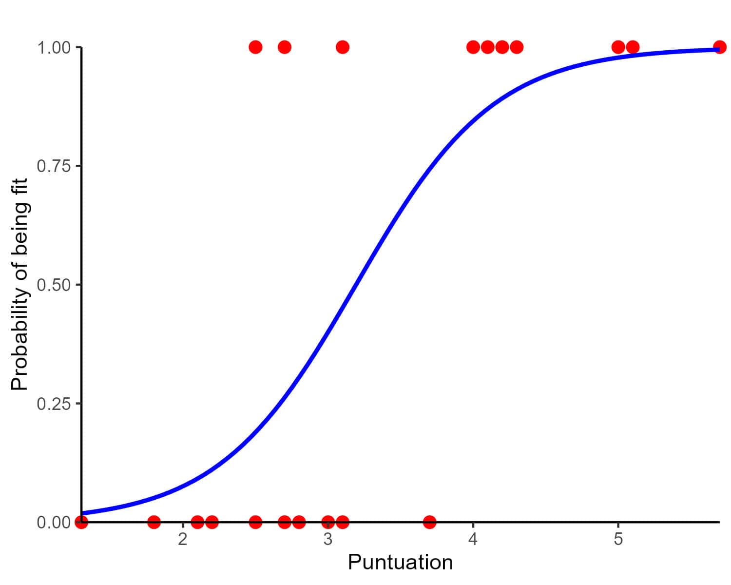
We can see a representation of the model in the attached figure. Using this figure, we could approximate what the probability of being “suitable” would be for a new candidate with a score of, say, 3.5: a little over 50%.

But we can get a more precise estimate by plugging the score into the model equation and using the sigmoid function to calculate the probability:

We already know that a candidate with a score of 3.5 will have a 65% chance of being “suitable” for the space program.

When binary is not enough

Our guys at NASA already know how to predict which astronaut candidates they can hire for the program. They would only have to reject those who, according to the previous model, had a probability lower than what they considered appropriate as a cut-off point.

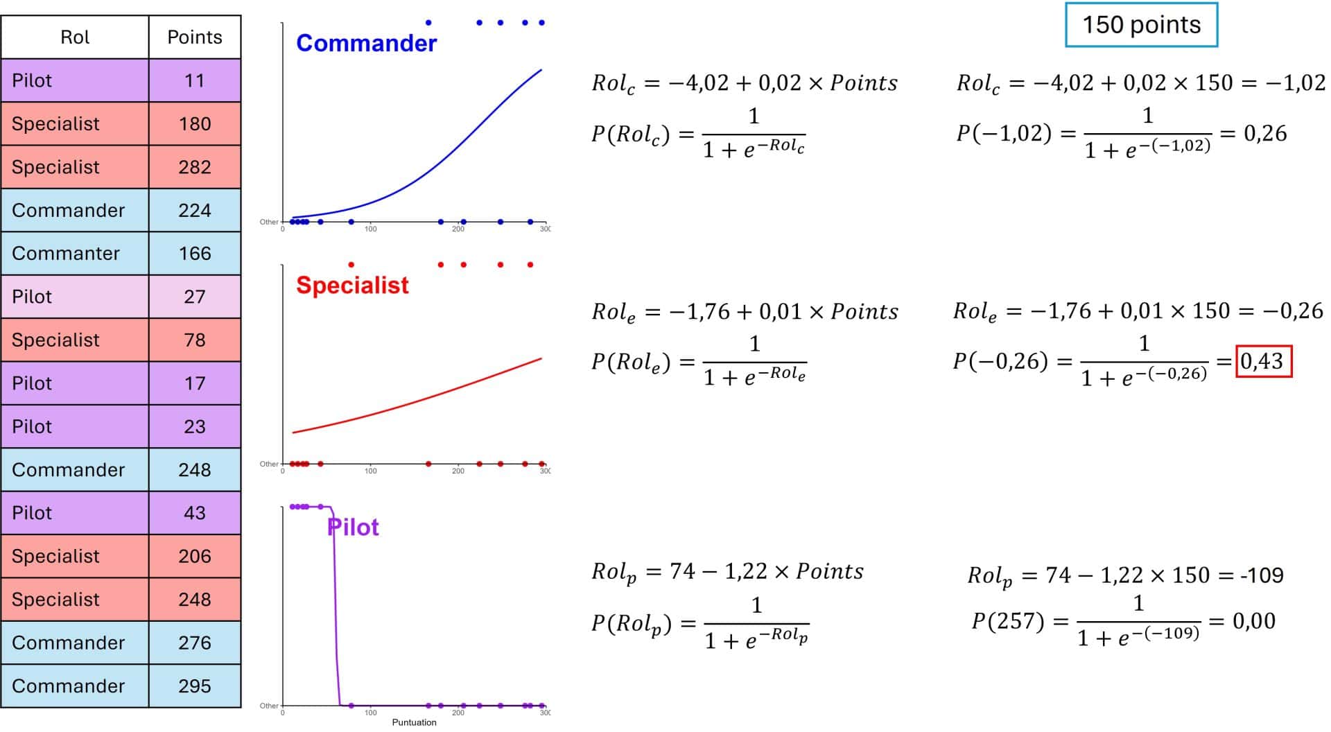
Now, once they have been admitted, they need to decide what role they will play during the flight: commander, mission specialist or pilot. To do this, they have another set of 15 astronauts with the results of another evaluation test, which you can see in the following figure.

The engineers, happy with the good result that the binary logistic regression model gave them, the first thing that occurs to them is to do something similar, but, since there are three categories in the variable that they want to predict (it is no longer binary), they opt for the so-called all-against-one strategy.

This consists of building three binary regression models, grouping two categories as one in each of the models. In the first, the target is coded as commander (1) or other (0). In the second one, specialist are coded by 1 and the combination of the other two by 0, and in the third, 1 is reserved for pilot and 0 for the other two combined. You can see the whole process in the figure above.

The first thing they do is calculate the three models. Once this is done, they consider which role would be the most suitable for an astronaut who obtains 150 points in the test. They substitute the score value for 150 and calculate the result for each case.

For example, in the case of the first model, that of commander, we obtain a value of -1.02. To calculate the probability that the commander role is the ideal one, we introduce this value in the logistic transformation equation that we did to build the logistic regression model, as we explained above.

The sigmoid function gives us a probability value of 0.26. Once this calculation has been made with the three models, we would choose the one that gives the maximum value, which in this case is the specialist, which gives us a value of 0.43.

In conclusion, if a candidate obtains this score in the test, the position for which he is most likely to perform a good job will be that of mission specialist. He might even be an acceptable commander, but he would certainly seem poorly suited to be the pilot of the mission.

At this point, you might think that the engineers have solved the problem elegantly, but the truth is that things can be done better. The problem is that they have calculated the position that might be the best for the candidate, but they cannot estimate with what probability.

If you notice, the values ​​given by the three models do not add up to 1, which means that they do not represent direct probabilities of belonging to each category of the variable that is to be predicted. To achieve this goal, when the variable has more than two categories, we cannot use the logistic or sigmoid function, as we did with binary variables. In these cases, we must resort to another slightly more complex function, the softmax function.

The extension beyond binary

The softmax function is a generalization of the sigmoid function that is useful for multiclass classification, since its objective is to convert the set of probability values ​​so that they add up to 1. This makes it easier to interpret the results in terms of categories.

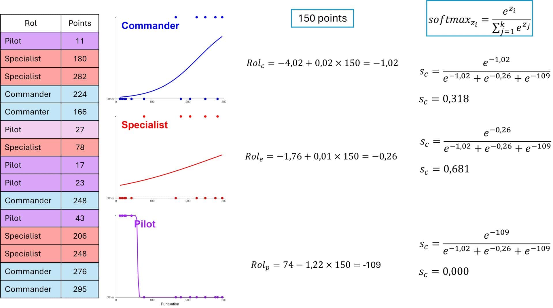
In the following figure you can see its expression. Unlike the sigmoid function, the softmax divides by the sum of the results of the three models (their log-odds).

Note that now, the results of the three categories add up to 1 (in reality they add up to 0.99, but you know, rounding problems). Now we know that the probability of a candidate with 150 points playing a good role as a specialist is 68%, a little more than double that of being a good commander. And, of course, don’t put him in the pilot’s seat.

Multinomial logistic regression

Everything we have seen so far serves to see how we can calculate the probabilities of belonging to a certain category of a nominal variable when we deal with variables of more than two categories.

From everything we have talked about arises the technique that is usually used when we need to do multiclass classification, which is none other than multinomial logistic regression.

Multinomial logistic regression calculates k-1 different models (where k is the number of categories of the variable to be predicted) so, in our example, we only have to adjust two models, since one of them will be taken as the reference model (we will soon see why only two and not three).

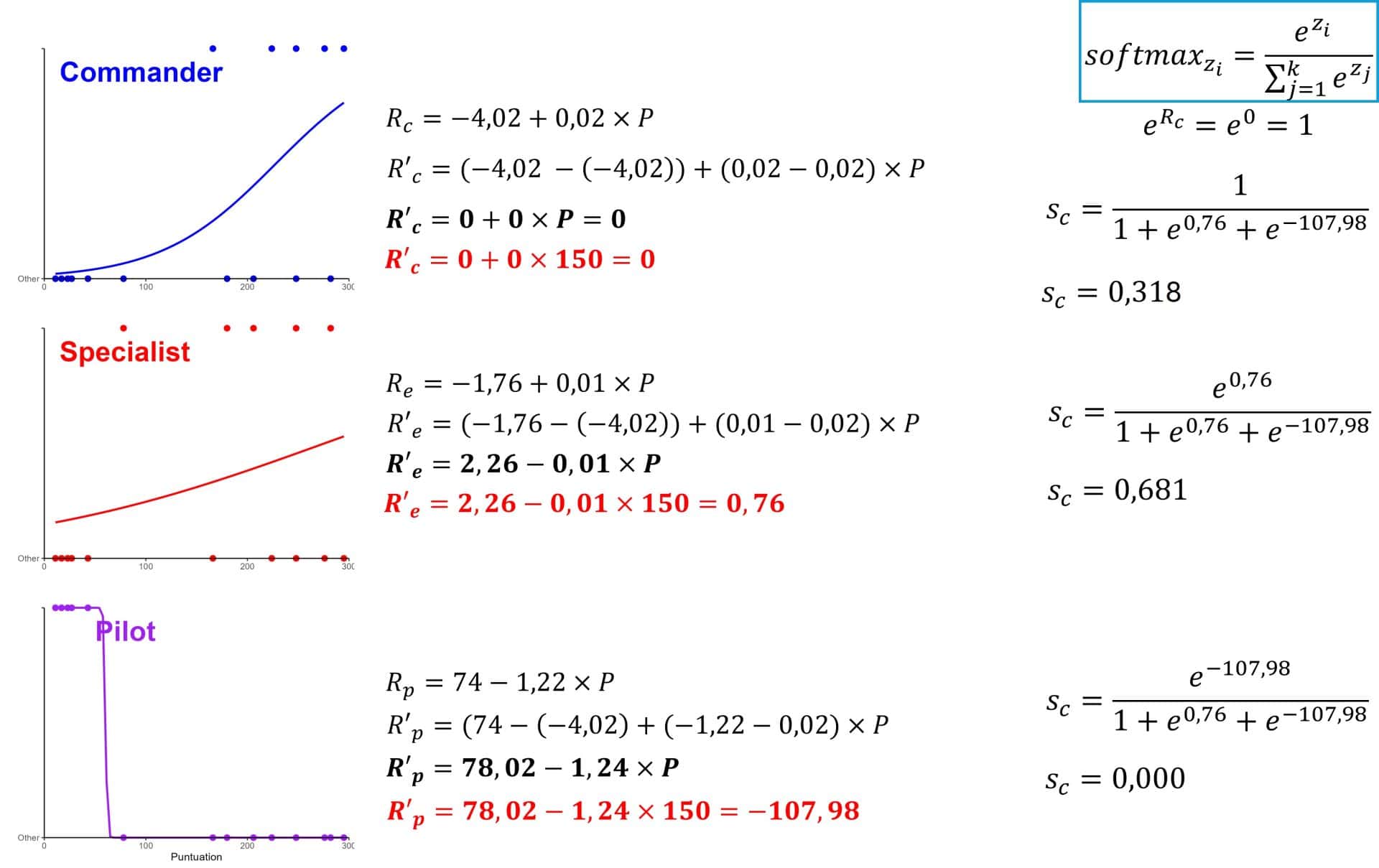
To do so, we subtract from each model the parameters of the model that we take as a reference, which in our case will be the commander model. You can see the calculations in the following figure.

Now, with the new models we can apply the softmax function to calculate the probabilities of each category for a score of 150. As expected, we get the same probability values but notice something interesting.

Since the log-odds of the reference model is 0, its contribution to the softmax function is e⁰ = 1. Therefore, the probabilities only depend on the log-odds of the other two models. This is what allows multinomial logistic regression to take a category as reference and fit k-1 models to estimate the k probabilities.

The quickest way

Needless to say, we have done all these calculations for fun, because when we have to solve a similar problem, we will resort to a statistical program that will do it in the blink of an eye.

I have done it with R. You can see it in the script that I mentioned at the beginning of this post.

To interpret the results of the program, we must take into account that it will give us the results of the specialist with respect to the commander and of the pilot with respect to the commander, separately (commander is used as a reference for both).

For example, for the specialist it tells us that the intercept is 2.83 and the coefficient for the score is -0.01. This coefficient tells us that the increase of one unit of the score decreases the probability of being a specialist compared to being a commander.

In addition, we can calculate the odds ratio by doing the antilogarithm of the coefficient. Thus e^-0.01 = 0.99. An odds ratio less than 1 tells us that the higher the score, the less likely it is that he will be a specialist and the more likely he will be a commander.

In summary, higher score values ​​are associated with a higher probability of being a future commander than a future mission specialist.

Of course, we can only conclude all this by validating the regression model, checking that it is significant and those details that we have not paid attention to because they are not the topic of today, but which are very important.

We’re leaving…

And here we leave this long space race for today.

We have seen how the sigmoid function, very useful for estimating probabilities in binary classification, does not allow the calculation of direct probabilities in multiclass classification, something that its extended version, the softmax function, is capable of.

And this does not only apply to logistic, binary or multinomial, regression, but also has its parallel in artificial neural networks that perform classification.

Indeed, the last layer of the network will choose sigmoid or softmax as the activation function, depending on whether binary or multiclass classification is performed. But that’s another story…