Neural networks.

The great Arthur C. Clarke said that any sufficiently advanced technology is indistinguishable from magic, suggesting that to someone who does not understand the underlying scientific principles of an advanced technology, this technology may seem magical or even miraculous.

And it is a reality that, as technology advances, it can be difficult for the general public to understand how it works, which can lead to a misperception of technology as something supernatural.

Something like this happens to us when we see how neural networks work. When we see autonomous driving cars, virtual assistants or image recognition algorithms in action, it seems like magic. But let’s not fool ourselves, there is nothing magical about them, they are based on the repetition of relatively simple operations.

What does seem magical to me is the ingenuity necessary to develop these ideas and how to make the scalability of simple processes reproduce results that, as Clarke said, seem magical or even truly miraculous to us.

We are going to try to discover the science behind the magic.

Neural networks

Neural networks receive this name because they are inspired by the structure and functioning of the human brain. In the same way that neurons are the basic cells of the brain and are interconnected in a complex network, artificial neural networks are designed with a large number of interconnected processing units called, how could it be otherwise, neurons.

These neurons are grouped into layers that are connected to each other. In general, there will be an input layer (where the data to be processed by the network is entered), one or more hidden or deep intermediate layers (where the data is processed) and an output layer (produces the final output of the network, which can be a classification, a prediction or a combination of both).

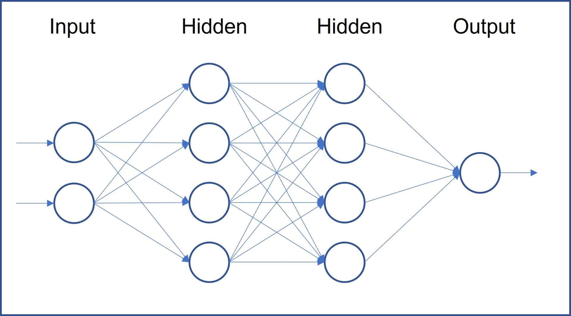
These layers are connected to each other, so that the output of one layer constitutes the input of the next layer, as you can see in the diagram in the first figure. There are several types of neural networks that are used for different purposes, some of the most common are:

• Forward propagation neural networks: they are the most common and simple type of neural networks, commonly used for classification and regression.

• Recurrent neural networks: they have backward connections between layers, which allows them to process sequential data, such as text or audio signals, and are often used to make predictions with time series (weather forecasts, etc.).

• Convolutional neural networks: they are designed to process data with high-dimensional structures, such as images, so they can be used for classification, recognition of objects within an image, etc.

• Generative neural networks: generate new data, such as images or text. This type of network is what is behind our partner chatGPT, the image generating algorithms and some other wonders.

• Self-encoding neural networks: they are used for dimension reduction, that is, to reduce the complexity of the data by extracting the most important features.

But there is something that all these networks have in common, and it is their basic unit: the neuron. Let’s see how it works.

The neuron

The neuron is the fundamental component of the neural network. You can see in the second figure the scheme of operation of an individual neuron.

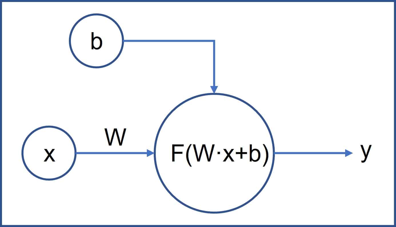
A neuron receives a series of inputs, performs an operation with them and generates an output, which will be the input of the neurons of the next layer (except in the last layer, whose output is the final result offered by the network).

Let’s assume the simplest example: we want to predict the value of a variable “y” based on another variable “x”.

The variable x would be one of the inputs of the input layer neuron. But this neuron also receives two parameters, one called weight (W) and another called bias (b).

In the case of the simplest networks, the operation carried out by the neuron is the vector product of the weight by the variable, to which the bias is added:

W · x + b

In a real example usually will there be many input variables (x₀, x₁, …, x_n), each accompanied by its corresponding weight (W₀, W_{1, …,} Wn). The point of the above equation represents the vector product of the two matrices (in neural networks, the matrices are called tensors). There is a lot of linear algebra behind the scene, but we don’t need to know it in depth to understand intuitively how the network works.

In the case of a variable and a network of a neuron, the result to predict the value of “y” could be expressed as follows:

y = W · x + b

The most attentive of you will have already thought that what the neuron does with the input variable is nothing more than a linear transformation (the equation is similar to that of simple linear regression). The problem is that this linearity causes us a small inconvenience.

We have said that neural networks are made up of successive layers of interconnected neurons in such a way that the output of one neuron is the input of the next. Now, if all the neurons do a linear transformation of their input, it won’t do us any good to chain layers of neurons together. And this is so because any number of successive linear transformations is equivalent to only one. We would gain nothing by chaining layers of neurons together.

The solution is that each neuron, once the previous operation has been carried out, before giving the output, performs one last non-linear transformation. In charge of this is the so-called activation function, which, in a display of creativity, we will call f. Thus, the equation of each neuron could be expressed as follows:

output = f(W · x + b)

And this function f already applies a nonlinear transformation, which allows us to detect complex nonlinear relationships between the data when we combine multiple layers of neurons.

There are several activation functions that can be used, depending on the data and the type of network used. For the most curious, I will tell you that the most frequent is the so-called ReLU (rectified linear unit), which leaves the result as it is if it is greater than zero or transforms it into zero if it has a negative value.

Searching for magic

So far we have seen what basically each neuron in the network does. We have given a simple example with one input variable, but in practice there will be many more: hundreds, thousands and even millions of them (to make things more complicated, there can also be more than one output, but let’s ignore this for simplicity).

We are going to try to understand how the network is able to predict the output value.

Initially we have a neural network model with a series of weights, depending on the number of input variables, which we will provide. Also, in our simple example, we need to provide the network with the true value of the variable that it has to predict. What the network does is (1) assigns the weights a random initial value (yes, a random value), (2) puts the weights and variables in the network and does the simple operations that each neuron has being programmed with, and, finally (3) compares the output value that it obtains with the true value of “y”, the variable that we want to predict.

As you can see, a neural network simply consists of a series of operations that make some transformations of the input data to generate an output data. The magic happens when you scale the model with multiple neurons and layers: it becomes a complex transformation of tensors inside a multidimensional space that we can’t even imagine. Of course, all this is done based on a succession of simple steps.

Winter comes

In the scheme we have seen so far, the network initializes the weights randomly, processes the input variables, and gives us an output. As anyone can understand, when we compare the output with the actual value of the variable we want to predict, they will surely be quite different.

It is logical, we have given a random value to the weights, when the objective of the model is to calculate (to learn) what should be the weight for each input variable to obtain an output that resembles the real value as closely as possible.

This comparison between the value predicted by the network and the real one is made by means of the so-called loss function. For example, if our network tries to predict the value of a quantitative variable, the loss function can be that of the least squares: it compares the differences between the prediction and the actual value, squares them (to avoid negative signs) and average them. We could also use the absolute value of the differences. In any case, we need to find the value of the model weights that minimizes the value of the cost function.

Now we just have to modify the weights and run the model again. In a real case, we will only have to manually modify thousands or millions of parameters and repeat the process to see what our loss value is.

This is, as is easy to understand, unfeasible from a practical point of view. The goal will be for the network itself to be able to do this automatically and learn which weight values are the most appropriate. It’s called machine learning for a reason.

The lack of a solution for this problem led to a period of more than 10 years of halt in the development of neural networks, a period popularly known as the winter of artificial intelligence.

But finally spring came, thanks to the development of two magic-named algorithms: backpropagation and stochastic gradient descent.

Stochastic gradient descend

We already know that the goal of the network is to analytically find a combination of weights that minimizes the value between the prediction and the true value. This is equivalent to saying that we need to find the minimum point of the loss function that we are using, as shown in the third figure.

Consider a model with a single variable as input. Its loss function is continuous and differentiable, which means that we can calculate the derivative for any value of the weight that we have used.

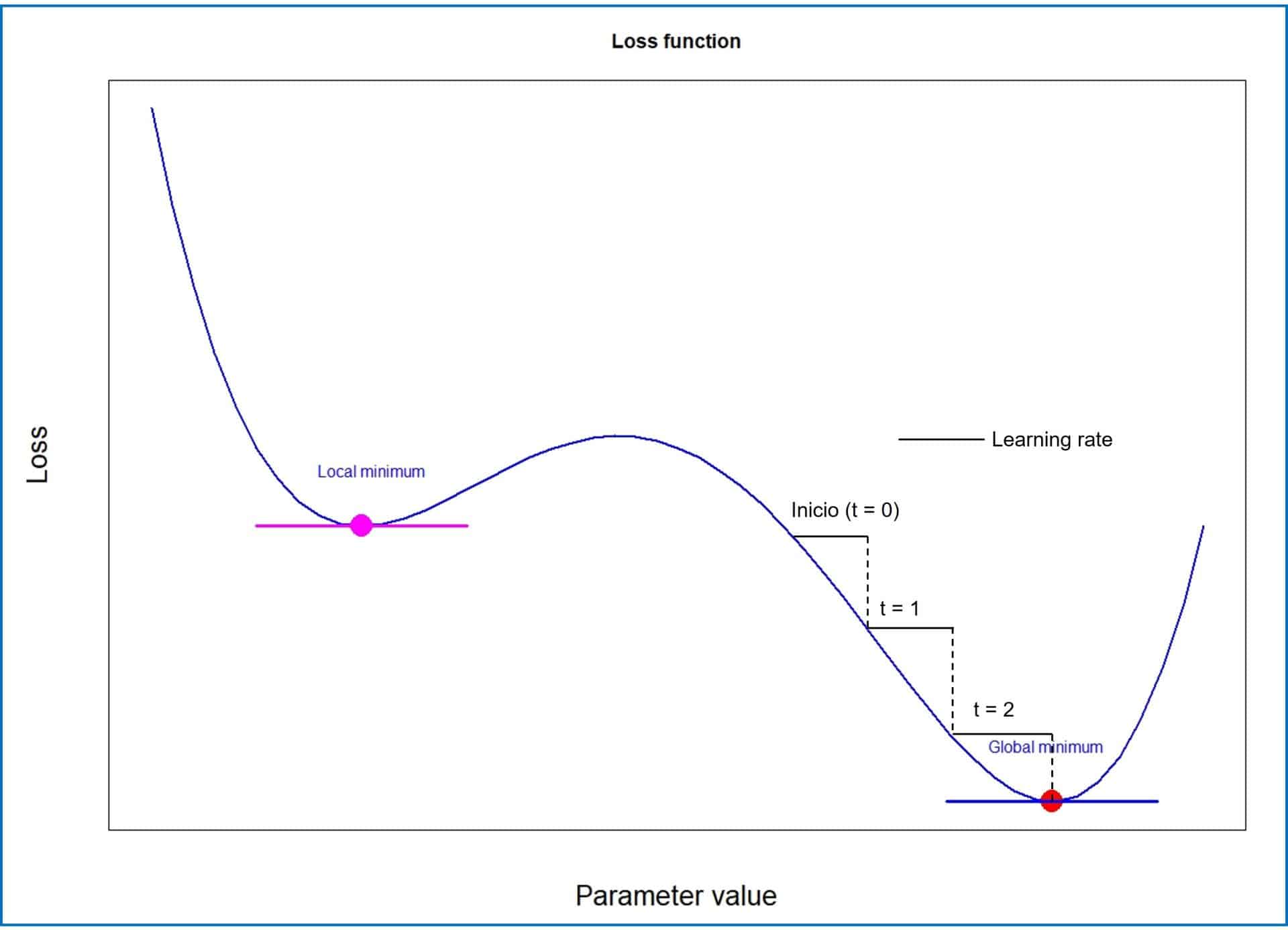
As we know from our school days, the derivative measures the slope of the function curve. When the derivative increases it means that the value of the function increases, and vice versa. At the minimum point of the function, the derivative will be zero.

Well, we already have it, we just have to go down the curve by modifying the weights of the model. To understand it better, we are going to draw a parallelism with an example of our adventurous daily life.

Imagine that you are teleported to a point in the Alps and told that you have to go to the deepest valley in the area. To make it easier, you don’t know the area, they cover your eyes and leave you at a randomly chosen point of the mountain range. How will you find the valley?

One way to do it could be the following: you take a couple of steps and feel with your foot where the terrain around you goes. You can thus know where it goes down and where it goes up. When you already know where it goes down with the steepest slope, you take another couple of steps and repeat the process. And so on until you reach the valley (or until you end up falling off a cliff at the bottom of a ravine).

In our neural network model, the slope is the loss function and our foot is the derivative. Actually, in a neural network model there are many input variables, so it will be necessary to calculate the partial derivative that corresponds to the weight of each variable. With these partial derivatives, a gradient vector will be obtained, which points towards the highest values of the curve. We already know in which direction we have to modify the weights: in the opposite direction that the gradient vector points to.

And how much do we change them? Here the equivalent of the number of steps we took in our example before testing the slope would come into play. The model uses a hyperparameter called the learning rate, which marks how much the weights have to be modified (the direction of the modification will be given by the gradient vector).

A very small or very large learning rate can cause the model to stagnate and never reach the minimum, or to err and reach a higher local minimum, like the one in the figure.

The model optimizer is in charge of all these calculations, which we will have to specify when we design the network. There are several types, such as RMSprop, Adam, Adamax, descending gradient with moment, etc, although we are not going to delve further into each of them.

Backpropagation

We have already solved the first problem for getting through the winter with the gradient descent algorithm. We know how we should modify the weights of the model to minimize the loss of the model, but we need the network to do it and learn by itself automatically. The backpropagation algorithm takes care of this.

The backpropagation algorithm is like the boss of a company who suddenly sees that there is a drop in the company’s sales volume. What he does is go department by department, in the opposite direction to the production chain, investigating the fault that each department has in the decline in sales and taking the appropriate measures in each one of them.

In a similar way, the backpropagation algorithm starts with the final loss value and works backwards, from the deepest to the shallowest neuron layers, calculating the contribution of each network node to the network loss value. Once this calculation is done, it adjusts the weights according to the learning rate in the opposite direction of the gradient vector calculated using the gradient descent algorithm.

Simple, right? With all that said, we can now assemble all the components to understand how a simple neural network works.

Assembling the network

In the fourth figure you can see schematized the operation of a neural network. The steps that the network follows are the following:

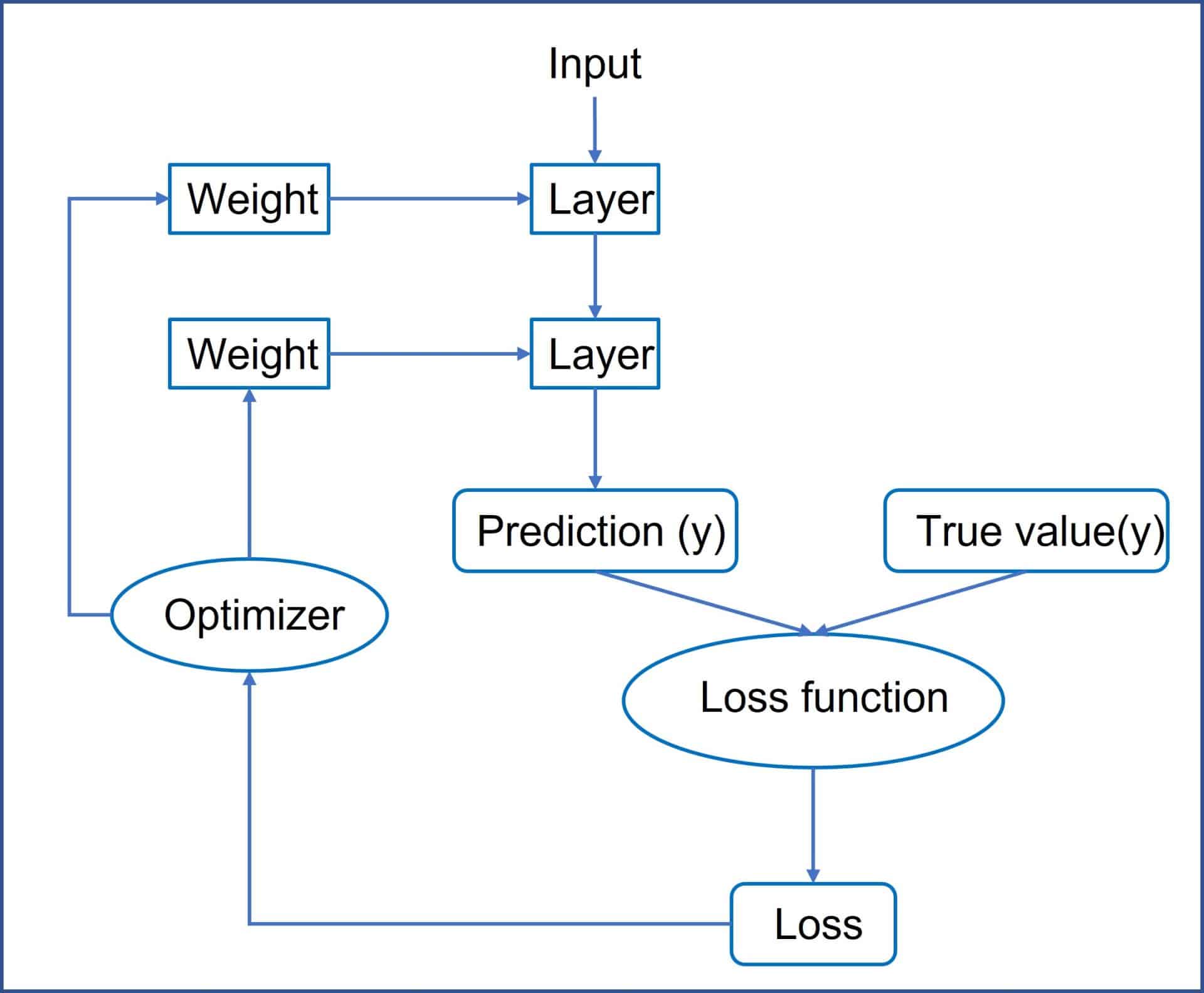
1. Take a set of input variables (x) and the corresponding real values of the variable we want to predict (y).

2. Run the model once (forward pass) to get the model predictions for the variable “y”.

3. Calculate the loss of the model, the difference between the actual values and the predictions.

4. Calculate the loss gradient at each node in the retrograde direction (backpropagation).

5. The weights are modified in the opposite direction to the gradient vector (multiplying them by the learning rate).

6. The model is executed again with the new weights, returning again to step 3 and repeating the cycle the necessary number of times so that the loss of the model is minimal.

All this process of trial and error constitutes the training of the network, during which it learns which are the values of the weights that minimize the los of the model. Each of these cycles is called an epoch, and each of these epochs can be done with all the data in the model or, more commonly, with portions of data called batches.

Once the model has been trained, it will be ready to predict the value of “y” from data with which it has not been in contact during the training phase and for which the real value of the variable is unknown.

We’re leaving…

I hope that, with everything said in this post, you have intuitively understood how an artificial neural network works and how they have nothing of magic and a lot of ingenuity and mathematical science.

In any case, I must confess to you that it still seems like something magical to me, even though I understand a little bit of the mathematical logic on which networks are based. We have only scratched the surface of how the simplest networks work. There are more types of connections, more types of networks, and more functions and techniques that can be used to optimize the performance of the network in this continuous struggle between overfitting and applicability or ability to predict results with unknown data. But that is another story…