Probability and linear regression.

Back in 1665, the physicist Christiaan Huygens, the guy who invented the pendulum clock, was lying in bed, recovering from an illness, when he noticed something weird: two pendulum clocks hanging from the same wooden beam started swinging in sync. He called it a “strange sympathy.”

At first, it just looked like a mechanical quirk. For a long time, people thought it was just a curious coincidence. But Huygens, ever the scientist, dug a little deeper and figured out that the clocks were subtly influencing each other through tiny vibrations traveling along their shared support beam.

What looked like random behaviour was actually the inevitable result of a sneaky little physical connection.

I bring this up because something similar happens with the famous practice of minimizing the sum of squared errors in linear regression. Most textbooks explain it like this: we square the errors to stop the positive and negative ones from cancelling each other out. You could just add up the absolute values of the errors, but squaring them has the perk of punishing big errors more than small ones.

That’s the usual textbook reason for using the sum of squares. And it’s not wrong, but it’s also not the full story.

Just like with Huygens’ pendulums, stopping at the surface explanation misses the deeper insight. Why squares? Why not cubes? Or some other power?

Here’s the real kicker: if we assume the residuals (those error terms) are random and normally distributed, minimizing the sum of squares isn’t just a convenient trick, it’s a mathematical must. Today we’re diving into how practical-looking decisions can be rooted in deep, inescapable principles that nudge us, gently but firmly, down a very specific path.

A probabilistic approach to linear regression

So, the classic intro to linear regression usually kicks off with a leap of faith: the “best” model is the one that minimizes the squared distances between the data points and the regression line (i.e., the model’s predictions). Those distances are the errors or residuals.

And while squaring the errors makes sense on the surface, there’s a richer story underneath. To get to it, we’ll take a probabilistic approach that sheds new light on the whole process.

The goal of linear regression is to predict a continuous dependent variable based on a weighted sum of independent variables. Those weights are the regression coefficients. Here’s the classic formula:

Linear regression means figuring out which set of coefficients (B) best fits the data.

The catch? That linear model isn’t perfect. There will always be differences between what the model predicts and what actually happens, thanks to noise from real-world randomness and unmodeled variables. So we rewrite the equation to include that noise (aka residuals):

In other words, linear regression is really about finding the set of coefficients (B) that best explains the data while accounting for the noise.

And here’s the twist: the kind of regression equation we end up with depends heavily on what we assume about that noise.

A very normal assumption

We now see that residuals play a central role in calculating regression coefficients.

Residuals can come from all sorts of places: measurement errors, unobserved variables, or just plain randomness. Whatever the source, they’re usually a mash-up of many small, independent effects.

Enter one of the cornerstones of statistics: the Central Limit Theorem. It tells us that when you sum a bunch of random influences, the result tends to follow a normal distribution.

So if we follow that logic, it makes sense to assume our residuals are normally distributed.

Chasing likelihood

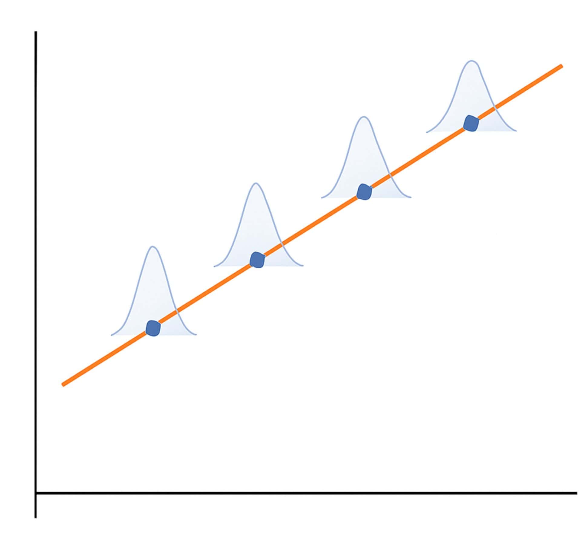
Now that we’re assuming normal residuals, we can say that each predicted point in our regression has some “cloud of uncertainty” around it: a bell curve centered on the ideal prediction. That curve tells us how likely a certain error is.

To keep things tidy, let’s use a bit of math-y notation. We’ll represent the probability of a data point given a set of model coefficients like this:

Here, B is our set of coefficients, X is the set of input variables (it’s a matrix of independent variables, hence the uppercase), and y is the output (just a single value, so lowercase).

This probability follows a normal distribution whose width depends on the coefficients. So for a given model, we can calculate the probability of seeing a particular error using the good old normal distribution formula (which we’ll skip here, for now).

If we go one step further, and assume each data point was sampled independently, then the probability of the whole dataset is just the product of the individual probabilities.

This probability of obtaining our dataset given a particular set of regression coefficients is what we call the likelihood of the model. If we’re comparing several models with different sets of coefficients, the better model is the one with the higher likelihood or, in other words, the one that makes the observed data more probable given its specific coefficients.

And take a moment to notice that we’ve made a pretty big shift in perspective. The goal in building the model is no longer to minimize errors, but to maximize the likelihood, to find the coefficients that make it most likely for the model to have generated the data we observed.
Let’s throw in a little formula to mark the occasion properly:

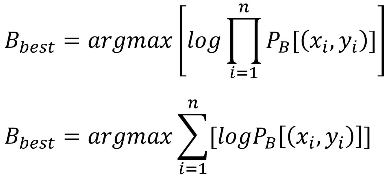
Let’s go a bit further. We can break that overall probability down into a product of the individual probabilities for each point.

All roads lead to Rome

We’re now in the final stretch of this journey, so we’re going to allow ourselves to complicate the math notation a bit (not too much) to fully wrap up what we set out to prove. You know what they say, a picture’s worth a thousand words (or so they claim).

Since the previous formula looks a little unfriendly and hard to work with, we’re going to simplify it, believe it or not, by applying logarithms to the right-hand side.

The big advantage of using logarithms is that the logarithm of a product equals the sum of the logarithms, and it’s much easier to work with sums than with products. The equation now looks like this:

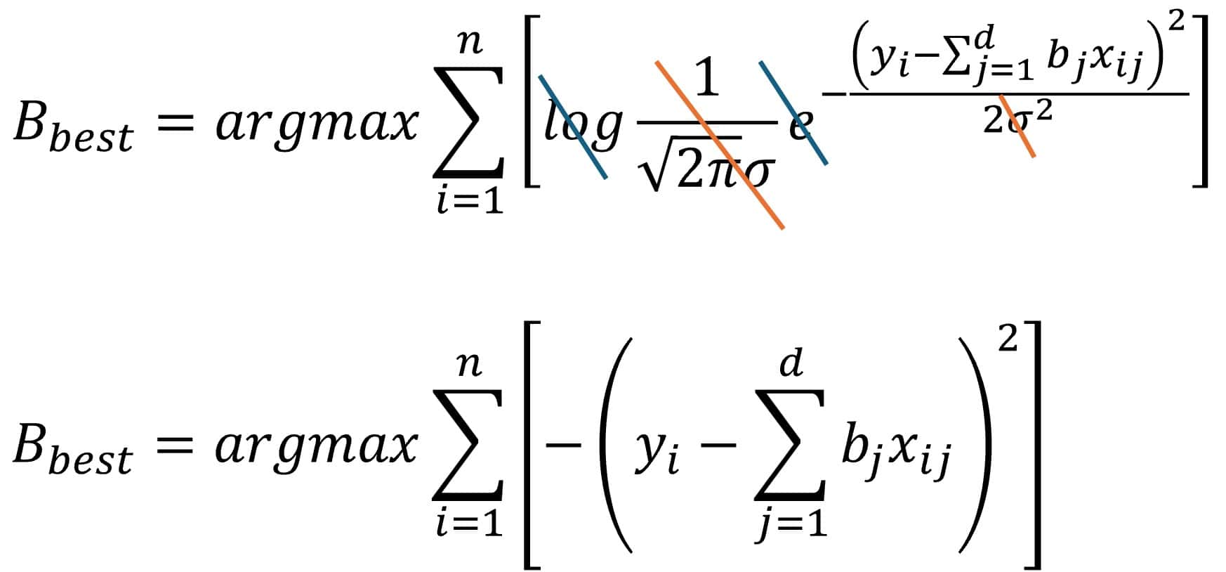
And now, don’t panic, we’re going to substitute the likelihood with its actual value according to the normal distribution equation, as shown below:

Please, don’t leave just yet. At this point, someone might be thinking I threw in that last formula purely out of sadism, but I swear that’s not the case.

First off, let’s clarify that the term “d” in the equation stands for the number of independent variables in the model. Now let’s take a closer look at the rest of the formula’s components.

Aside from our data and our coefficients, every part of the normal distribution formula is a constant, except for the standard deviation, sigma. But sigma doesn’t affect which set of coefficients will maximize the model’s likelihood, since it’s a fixed value and doesn’t play a role in the optimization process.

So, in short, we can simplify the equation by getting rid of sigma and the other constants (since they don’t matter for optimization), along with the logarithm, which cancels out with the exponential (everything raised to the power of e). Pay close attention to what we’re left with:

According to this formula, the optimal coefficients are the ones that maximize the negative sum of the squared differences between the linear fit and the observed points, in other words, the sum of squared residuals.

To shed light on what might still look a bit obscure, we’re going to make one last transformation to the equation so we’re working with positive error values, which, logically, we want to minimize. (And really, maximizing the negative of a value or minimizing the positive of that same value amounts to the same thing):

Once again, all roads lead to Rome. If we start from the assumption that residuals follow a normal distribution and eliminate everything that doesn’t affect model optimization, what magically emerges is… the famous least squares formula!

To put it a little more elegantly, we’ve seen that maximizing the log-likelihood is equivalent to minimizing the sum of the squared residuals.

We’re leaving…

And with that, I’ll say goodbye—for today—to those of you still reading this post (assuming there’s anyone left).

We’ve seen that we don’t square the residuals because it’s easier or somehow fairer. We do it because it’s what has to be done if we assume the residuals follow a normal distribution, which is a key assumption that needs to hold if we want to use linear regression properly.

Minimizing the sum of squares is just another way of maximizing the likelihood under that assumption. And that’s why, even if it might seem like a quirky tradition, there’s a whole mathematical logic choreographing this dance. The square is a direct consequence of assuming the errors are normally distributed.

Just like Huygens’ pendulums, which seemed to sync up out of mechanical courtesy, our statistical models also fall into rhythm… but with the bell curve of Gauss. When everything resonates at the same frequency, something almost magical happens: the model doesn’t just work: it sometimes even makes sense.

And if you thought this was the most elegant thing linear regression had to offer, just wait until we start penalizing overly enthusiastic models. Because yes, the choice of regularization terms (like ridge or lasso) also has a probabilistic explanation, incorporating our prior beliefs about how the model should behave, in pure Bayesian style. But that’s another story…