Regression regularization techniques.

It seems to me that lately I’ve been spending more time than I should have wandering into a faraway and mysterious corner of the world of statistics, where an epic dance is taking place that has left many connoisseurs stumped and, at times, reeling. That corner I am referring to is that of multiple regression, where the numbers dance to the rhythm of the data and the equations get entangled in a mathemagical whirlwind.

No one will be surprised, then, that when I fall asleep, I am assaulted by unreal and distressing nightmares, worthy of a dark Lovecraft’s story. Without going any further, the other night I dreamed that I was attending a fancy data party. The numbers were dressed in their best Gaussian garb, the equations chatted in groups, and the independent variables tried to impress the dependent ones.

In the center of the dance floor, the DJ was spinning probability distribution records while regression models made their grand entrance. It is at that moment when my gaze was fixed in one of the corners of the room, attracted by a dazzling couple. She was the star of the night, the diva of gradient descent, the queen of regularization. With her penalty outfit and her restraint demeanor, the LASSO Regularization was joined by Ridge, the intense-eyed hunk who slid into less overfitted models. Both were preparing to enter the dance floor.

I woke up with a start and drenched in sweat, gasping for air. I found it impossible to get back to sleep that night, so I began to investigate how my models could find the balance between the extravagance of overfitting and the rigidity of undercutting. If any of you are interested in knowing the results of this delusion, I invite you to continue reading this post.

The tribulations of multiple regression

Linear regression is a statistical method for modeling the relationship between a dependent variable and one or more independent variables. The goal is to find the equation that best fits the data to predict the values of the dependent variable based on the values of the independent variables.

Usually, this is achieved by the method of least squares (also called ordinary least squares), which tries to minimize the differences between the observed values of the dependent variable and the values predicted by the model, differences that are known by the name of residuals. The residuals are squared (so that the positives do not cancel out with the negatives) and added. The best regression equation will be the one in which this sum of the squares of the residuals has the lowest value.

Although this method produces a model that has a good fit to the data with which it has been built, it may not be as good when trying to predict the values of the independent variable with new data, different from those used during its construction. This can occur when a series of circumstances occur.

The first is collinearity, which occurs when there is a high correlation between the predictor or independent variables. This can cause some of the regression coefficients to take excessively high or low values, with the opposite sign to what we might expect based on our knowledge of the model, or with remarkably high standard errors. In this situation, even if we are lucky that the model can make roughly correct predictions, it will be difficult to interpret it and the importance of each variable in explaining global variability.

Another problem that can arise is that of high dimensionality or, put more simply, the existence of a large number of independent variables in the model. In general, more complex models have a tendency to overfit the data: they fit well with known data but fail to generalize to new data.

This reaches the limit if the number of independent variables is close to the number of participants (sample size), in which the method of least squares may fail to obtain the regression coefficients.

Well, to alleviate or solve these problems, we have a series of regularization or shrinkage techniques. Do you remember my dream and the couple that made me wake up? Well, yes, these two techniques are ridge regularization and lasso regularization.

Well, there is also a third one that shares the inheritance of these two: elastic net regularization. Let’s see what they consist of.

Regularization techniques

Regularization techniques help us to minimize the problems that we have described by placing restrictions on the regression coefficients of the model, which helps to control its complexity and prevent the coefficients from taking extreme values.

As we have already said, the two most common regularization techniques are ridge regression, also called L2 regularization, and lasso regression (Least Absolute Shrinkage and Selection Operator), or L1 regularization.

Both techniques are based on performing a modification of the ordinary least squares method by adding a penalty to the sum of the squares of the residuals. This results in a constraint or shrinkage on the model’s coefficients, which helps control its complexity, increases the stability of the coefficients, and avoids their extreme values.

Ridge regression

Ridge regression tries to minimize the prediction error by adding, to the original cost function (sum of the squares of the residuals), a penalty term proportional to the square of the coefficients. The formula would be the following:

Modified cost function = original cost + λ x Σ(coefficients²)

The value of the parameter λ is determined by the researcher and must be greater than zero, since if λ = 0 there is no difference with the multiple linear regression without regularization. The larger the value of λ, the greater the constraint that is placed on the model.

If we think about it a bit, squaring the coefficients penalizes the coefficients with a higher value more. The result when, for example, there is collinearity, is to approximate the extreme values to intermediate values. The coefficients are close to zero, but without reaching this value (as we will see what happens in the lasso regression), so they do not disappear from the equation, although their impact on the global model does decrease.

Lasso regression

Lasso regression also adds a penalty term to the original cost function, but in this case, it is proportional to the absolute value of the coefficients and not to their squared value:

Modified cost function = original cost + λ x Σ|coefficients|

Lasso regression restricts the magnitude of the regression coefficients, but, unlike ridge regression, they can reach zero, which means that they disappear from the model. This is very useful to reduce the complexity of the model and when it is necessary to reduce the dimensionality, which is nothing more than to reduce the number of independent variables.

Again, when λ = 0, the result is equivalent to that of a linear ordinary least squares model. As the value of λ increases, the greater the penalty and more predictor variables can be excluded from the model.

Differences between ridge regression and lasso regression

Although both techniques decrease the magnitude of the regression coefficients, only lasso regression achieves that some are exactly zero, which makes it possible to select predictor variables. This is the greatest advantage of lasso regression when we work with scenarios in which not all the predictor variables are important to the model, and we want the less influential ones to be excluded.

For its part, ridge regression is more useful when there is collinearity between independent variables, since it reduces the influence of all of them at the same time and proportionally. We can also use it if we are faced with a situation in which losing independent variables is a luxury that we cannot afford.

However, we can find situations in which we are not clear about which of the two techniques to use or in which we want to take advantage of both. To achieve a balance between the properties of the two, we can resort to what is known as elastic net regression.

Elastic net regression: the midpoint

This technique combines the penalty of the L1 and L2 regularization techniques, which tries to take advantage of both and avoid some of their drawbacks. The formula would be the following:

New cost function = original cost + [(1 – α) x λ x Σ(coefficients²)] + (α x λ x Σ|coefficients|)

To understand it a little better, we can write it more simplified:

New cost function = original cost + (1 – α) L1 penalty + α x L2 penalty

As you can see, we now have two coefficients, α and λ. The values of α oscillate between 0 and 1. When α = 0, the technique would be equivalent to doing a ridge regression, while, when α = 1, it would work like a lasso regression. Intermediate values would mark an equilibrium position between the two regularization techniques.

So, it is easy to understand that we have to decide the values of α and λ to know what degree of penalty to apply and what predominance of the two techniques to use. This is usually done by testing many values and seeing which one gives us the best results, a process that is usually taken care of by the statistical programs that we use for these techniques.

A practical example

I think it’s time to give a practical example of everything we’ve talked about so far. It will allow us to understand it better and understand how it is done in practice. To do this, we are going to use a specific statistical software, the R program, and one of its most used data sets for teaching purposes, mtcars.

This data set contains information about different car models and their characteristics. It includes 32 rows (one for each car model) and 11 columns representing various car characteristics such as fuel efficiency (mpg), number of cylinders (cyl), displacement (disp), engine horsepower (hp), rear axle ratio (drat), weight (wt), quarter mile time (qsec), etc.

I’m not going to detail all the commands that need to be executed for this example, since this dance could go on until the wee hours of the morning, but if anyone is interested in reproducing the exercise, they can download the complete script at this link.

Let’s see the process step by step.

1. Loading function libraries and data preparation.

In R, the first thing we do is load the libraries that we are going to need for data processing, its graphic representation and the development of multiple linear regression models and regularization techniques.

Next, we load the data set. We prepare a vector with the dependent variable and a matrix with the independent ones, since we are going to need them to apply the functions that perform the regularization.

2. Linear regression model.

We begin by developing the linear regression model taking engine horsepower (hp) as the dependent variable and the rest of the variables as independent or predictors.

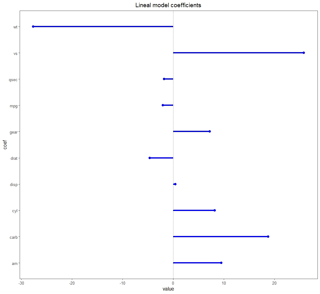
Focusing on the results that interest us for our example, the model is statistically significant (F = 19.5 with 10 and 21 df, p < 0.05) and explains 85% of the variance of the dependent variable (adjusted R² = 0, 85). But the most interesting thing is to look at the attached figure with the regression coefficients.

You can see that there are some that draw attention due to their magnitude compared to the others, such as those of the wt and ws variables.

This may be a sign that collinearity exists. In addition, the model has a large number of predictor variables for the sample size (only 32 records), so the risk of overfitting is high. We decided to apply regularization techniques.

3. Ridge regression.

If we use R, we can perform regularization techniques with the glmnet() function, adjusting the value of its alpha parameter. To make it perform a ridge regression, we set the value of alpha = 0.

We have already said that we have to choose the value of λ that we are interested in applying. And how do we know? R helps us in this task. The glmnet() function does not calculate a single model, but many (100, if we don’t tell it otherwise) with different values of λ. Each of these models will have different regression coefficients, as you can see in the next figure.

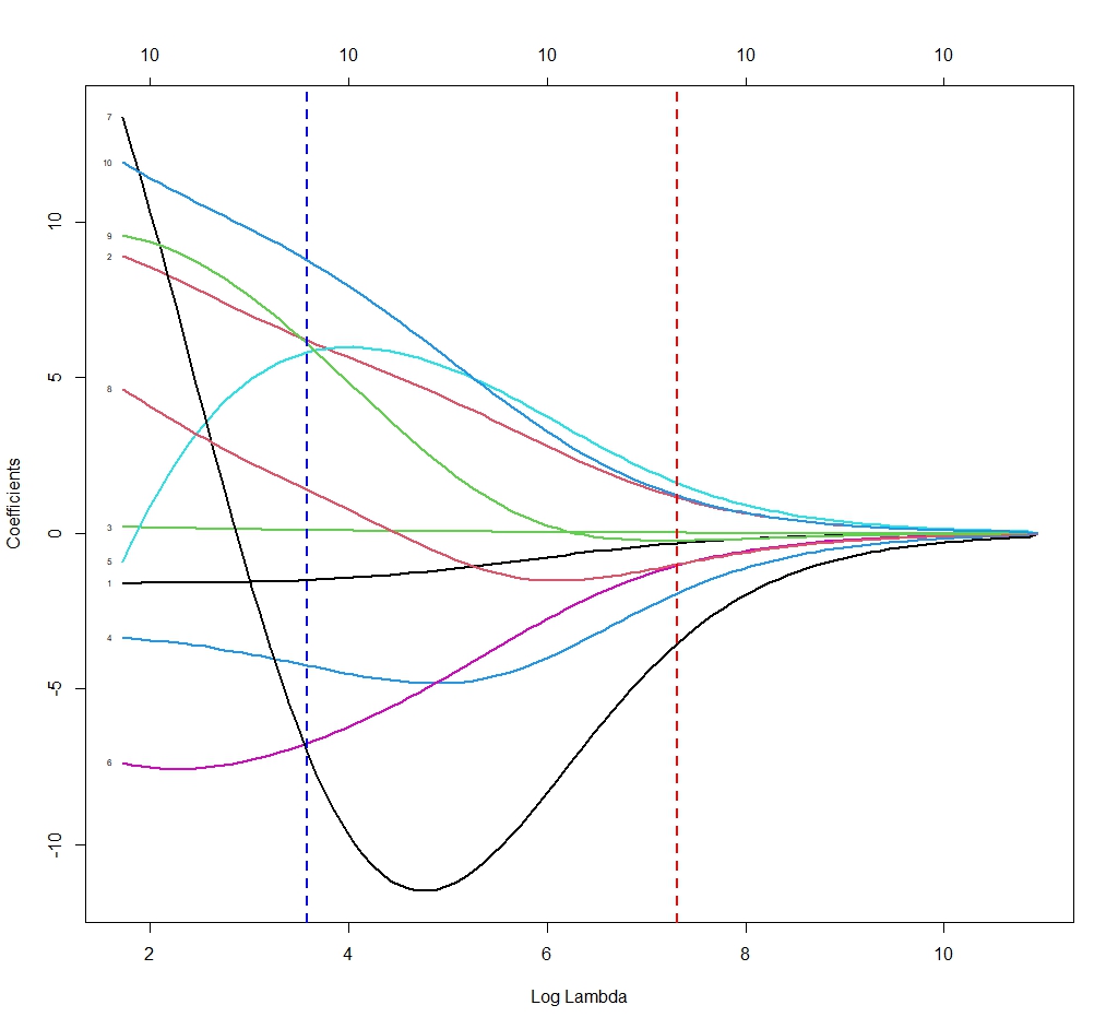
Each line of the graph shows how the regression coefficient of each variable varies as a function of the value of λ. For example, the blue line shows the values for λ = 80 and the red line for λ = 40.

The function also accounts for the cost function of each of the models and gives us two values of interest. One, the so-called minimum λ (λmin), which corresponds to the minimum value of the prediction error of the model. Two, the λ corresponding to a prediction error of one standard deviation from the mean of all the models (λ1se).

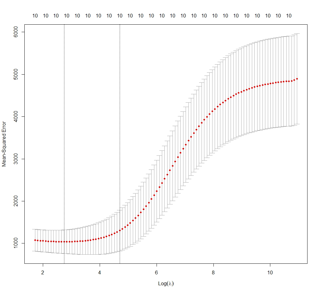
We are going to take the value of λmin (some people think that with λ1se there is less risk of overfitting). In the third figure you can see the distribution of the error of the model as a function of the value of the natural logarithm of λ. It marks the optimal limits between the two vertical lines. We choose our value of λmin = 17.

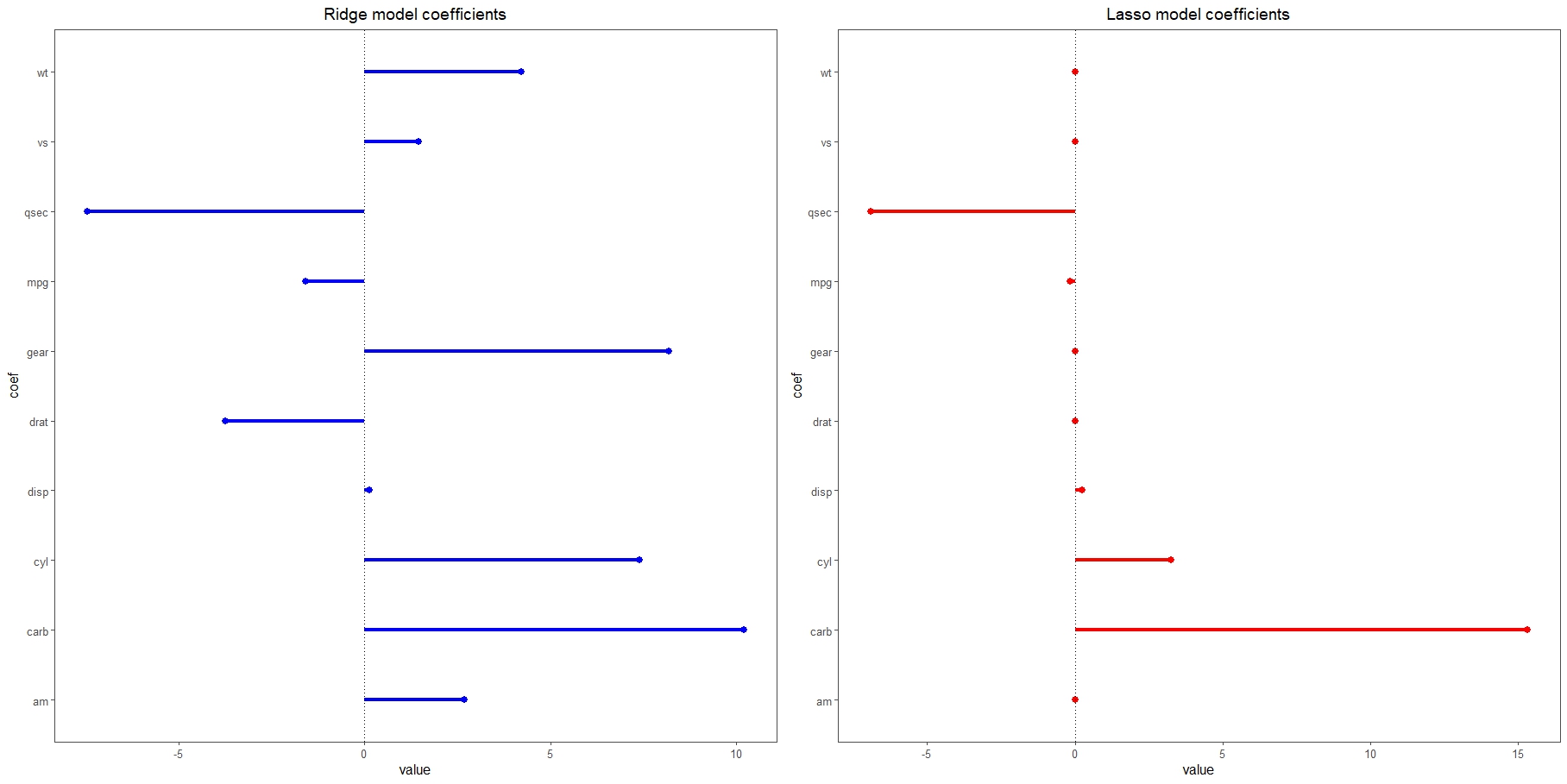
Look at the fourth figure in the distribution of the coefficients of the model corresponding to λ = 17 (which appear next to those of the lasso regression model that we will develop later). We can verify how the dispersion is less and how the magnitude of the coefficients has also decreased (if you compare it with those of the linear regression model, keep in mind that the scales are different, since visually they may appear very similar).

Now we only have to extract the values of the regression coefficients (it is of no interest for what we are dealing with). The model explains 85% of the variance of the dependent variable (R² = 0.87). If we calculate its error by the method of least squares, it is 24.5.

4. Lasso regression.

We would repeat the entire process of the previous step, but setting alpha = 1 in the glmnet() function.

We obtain a value of λmin = 17. The distribution of the regression coefficients is shown in the figure above. It is striking how 6 of them have become 0, with which they would disappear from the model. This is, as we already know, one of the characteristics of this technique.

If we calculate the performance of the model, we see that it is like that of the ridge regression, with a value of R² = 0.87 and a least-squares error of 24.02. We will have to decide which of the two interests us more, considering that, in this case, the point that we could take advantage of is the reduction of dimensionality provided by lasso regression.

5. Elastic net regression.

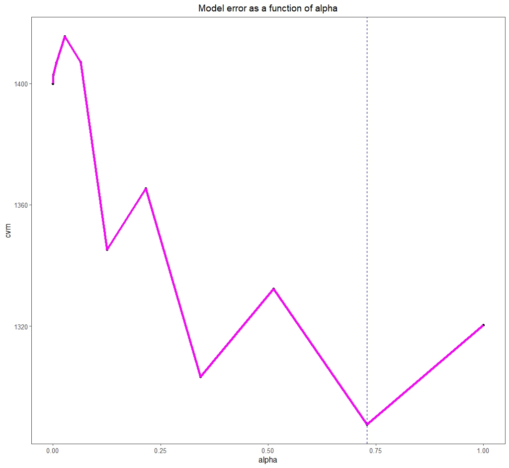
In this case we have to test models with multiple values of α and λ. This is done in R using the cva.glmnet() function, which employs cross-validation techniques.

This function tests several values of α (11, if we don’t tell it otherwise) and, for each of them, multiples of λ. Thus, in a similar way to the previous steps, we can choose the best value of α and, for this, the value of λ (in this case λ1se) that minimizes the model error, as you can see in the last figure.

We see that the optimal α value is 0.73. This marks the point between the two regularization techniques, L1 and L2, in which we will perform the best fit.

We are leaving…

And with this we are going to finish for today.

We have seen how multiple regression regularization techniques can be very useful when we have collinearity or overfitting problems. In addition, they can be used to select the independent variables and reduce multidimensionality, achieving more robust and easy-to-interpret models.

Before we say goodbye, I want to clarify that everything we have said is also valid for multiple logistic regression. The way to do it is similar, although there may be some small difference in the use of the statistical program that we use.

In the case of logistic regression, regularization is also useful when what is called separation or quasi-separation occurs, which takes place when the variables overfit a subset of the data available to develop the model. But that is another story…