Decision trees.

Last night I dreamed I went to Manderley again. I was in front of the gate, but for a few moments I couldn’t get in…

Well, actually, that didn’t happen to me, but to Rebeca, as film or literature fans will have already recognized.

I, in fact, had one of my Lovecraftian dreams again in which I found myself lost in a labyrinth in the land of numbers. There I was, submerged in a sea of unknown dimensions, where the predictor variables were intertwined in a chaotic dance of uncertainty. There was no way out of the maze: each corner led me to a new dimension of possibilities, and no exit seemed in sight.

If I had remembered Rebecca in my dream, I could have felt endowed with supernatural strength and crossed the walls of the labyrinth like a spirit. But of course, a squared and unpoetic mind like mine, could only resort to a much more pragmatic tool, although no less original within my dream universe.

So, I began to develop a decision tree that could turn the forks of the maze into clear and defined options and whose branches would extend, like Ariadne’s threads, guiding me through the enigma of variables towards a clarity that previously seemed unattainable.

The tree was my salvation compass in the multidimensional universe in which I found myself, leading me step by step towards the exit from the labyrinth of predictor variables. Thus, I escaped from the labyrinth of my dreams. When I woke up, I realized that if you use the right tool, even in the strangest and most unknown worlds, there is always a way to find the path to clarity and certainty.

And since I imagine that, after this rambling, you will be wanting to know what decision trees are and how they work, I invite you to continue reading this post.

Decision trees

A decision tree is a machine learning model that is used to classify or predict a target variable based on several input variables.

The trees work by stratifying the space of the predictor variables in a series of zones or regions. Maintaining the simile of gardening, the work system would be more like the way of dividing the data garden into plots so that, upon having new data, the prediction for that value with that set of predictor variables is the average value of the target variable of that plot.

This is shown graphically in the form of a tree, where each internal node represents a characteristic that allows us to separate each plot and each branch represents a decision based on that characteristic. Finally, each leaf or terminal node represents the result of the final decision or classification. And, I haven’t told you, the tree is drawn upside down, with the root on top and the leaves at the bottom.

To understand it better, we are going to give an example using the “mtcars” data set, which is frequently used for teaching with R, which contains information about different car models and their characteristics. It includes 32 rows (one for each model) and 11 columns representing various characteristics of cars, such as fuel efficiency (mpg), number of cylinders (cyl), displacement (disp), engine power (hp), the rear axle ratio (drat), the weight (wt), etc.

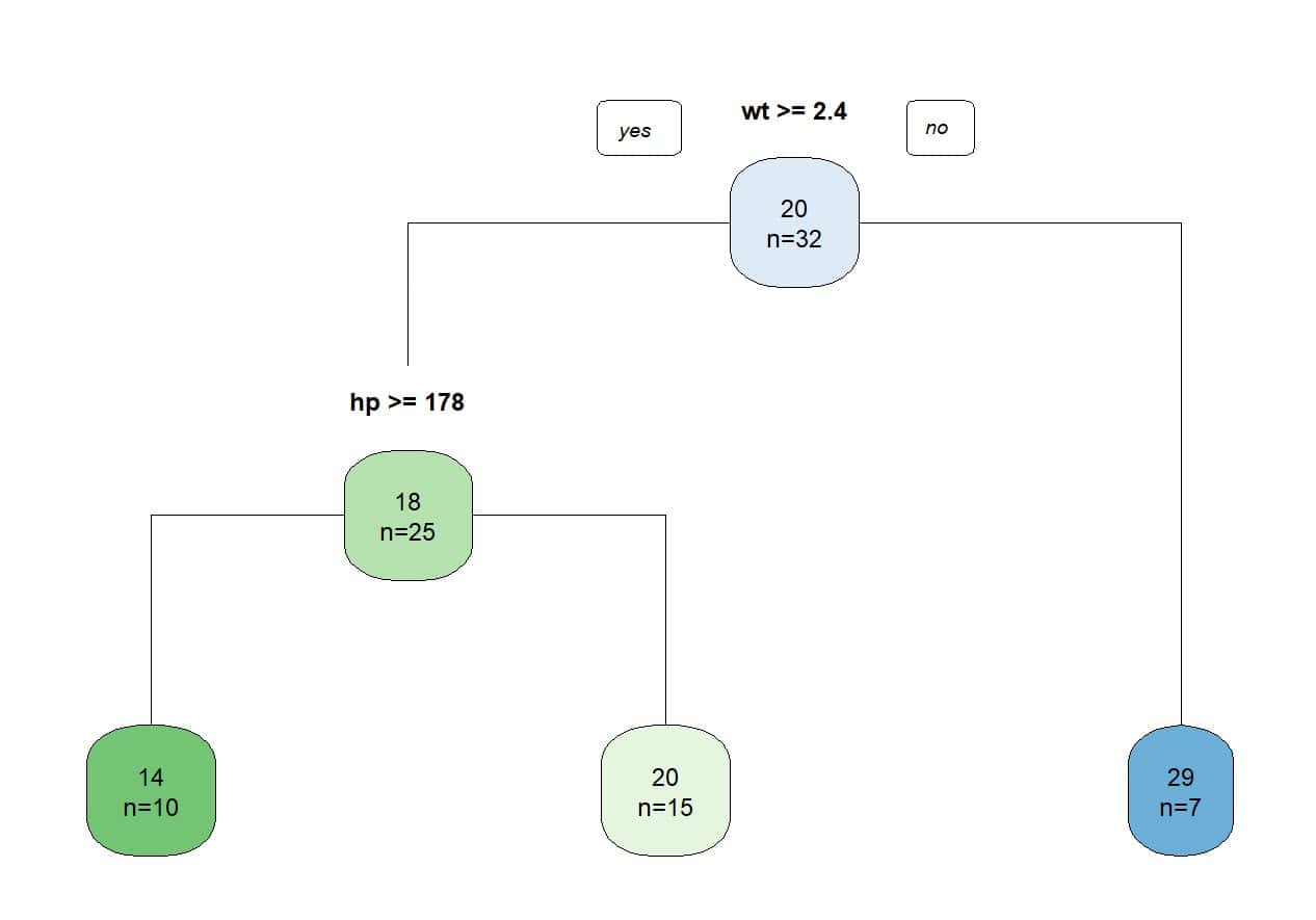
Suppose we want to predict fuel efficiency (miles per gallon, mpg) using the independent variables weight (wt) and engine power (hp). In the attached figure you can see the simple decision tree that we created with the R program.

The first thing we look at is if the weight of the car is equal to or greater than 2400 pounds. If the car weighs less than that amount, it will be able to travel, on average, 29 miles on one gallon of fuel. Engine power matters less in this group of lighter cars.

But if the car weighs more than 2,400 pounds, its power does matter. Those with less than 178 horsepower will travel, on average, 20 miles per gallon, while those with more than 178 horsepower will consume more fuel and have less efficiency: only 14 miles per gallon of fuel, on average.

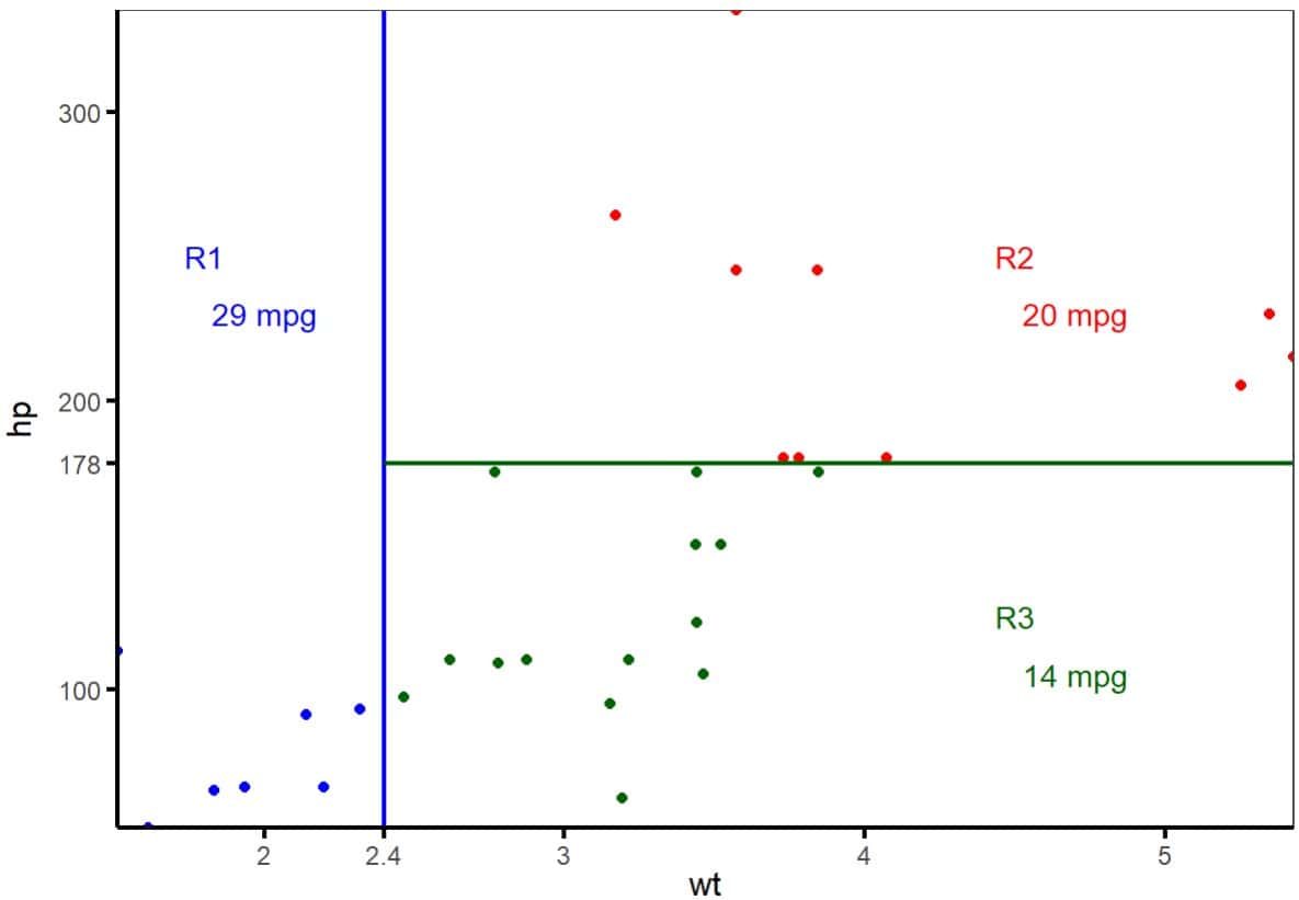
We see one of the great advantages of decision trees, which is their easy interpretation (especially if there are few variables and the tree is not very leafy). But, in reality, what the model does is divide the space of predictor variables into plots, as you can see in the second figure.

Initially it delimits a first region (R1) for the weight of less than 2400 pounds. The average efficiency of cars in this region is 29 mpg. The remaining space is, in turn, divided into two other regions (R2 and R3) according to the limit of 178 horsepower, marking the two groups with an average consumption of 20 and 14 mpg, respectively.

Once we have a new car for which we want to estimate its energy efficiency, we will only have to apply this system and assign it to the zone to which it belongs. Thus, the prediction of its energy efficiency will be that of the average value of the area to which it corresponds.

Logically, the more variables that are included in the model, the more we can refine the predictions. This example is very simple to be able to graphically show how we divide a two-dimensional space and better understand the concept, but, in our day to day, we will handle multidimensional spaces of predictor variables to estimate the value of the target variable of the new data that we want to estimate.

The next thing we are going to consider is how the regions are calculated to build the decision tree. Let’s see it.

Building trees

We have already seen that the objective is to divide the space of predictor variables into a series of multidimensional boxes or regions, so that new elements are assigned the average value of the region to which they belong. How do we know which regions are the best?

To calculate these regions, a very beloved system in the world of statistics and data science algorithms and models is used: a variation of the least squares method.

The tree is created with a data set for which both the predictor variables and the target variable that we want to estimate are known. Once the model is built, we compare the values that the tree predicts with the actual values.

The differences in these values (the residuals) are squared and added, much as is done, for example, to estimate the coefficients of a linear regression model. First, a sum is obtained for each region, and then the sums for all regions are added to obtain the sum of squares.

The objective will be to find the tree with which the lowest value of this sum of squares is obtained. The problem is that it would be computationally very expensive to calculate the sums of squares of all possible trees (with all combinations of the predictor variables in the different regions).

To solve this problem, a greedy approach is carried out  which, starting from the top-down, makes optimal local decisions at each step without considering the global consequences, with the aim of finding a generally acceptable solution at that point.

Thus, it begins by considering all the predictors and all their possible cut-off points, calculating the sums of squares of the residuals and selecting the one with the minimum value. Here the first partition of the space of the predictor variables is carried out.

This is then repeated recursively, generating the rest of the regions, equivalent to the branches emerging from each node of the tree. The approach is called “greedy” because it chooses each partition at a time when it is favourable, but without considering whether it would be better to use this criterion further down the tree.

Pruning the tree

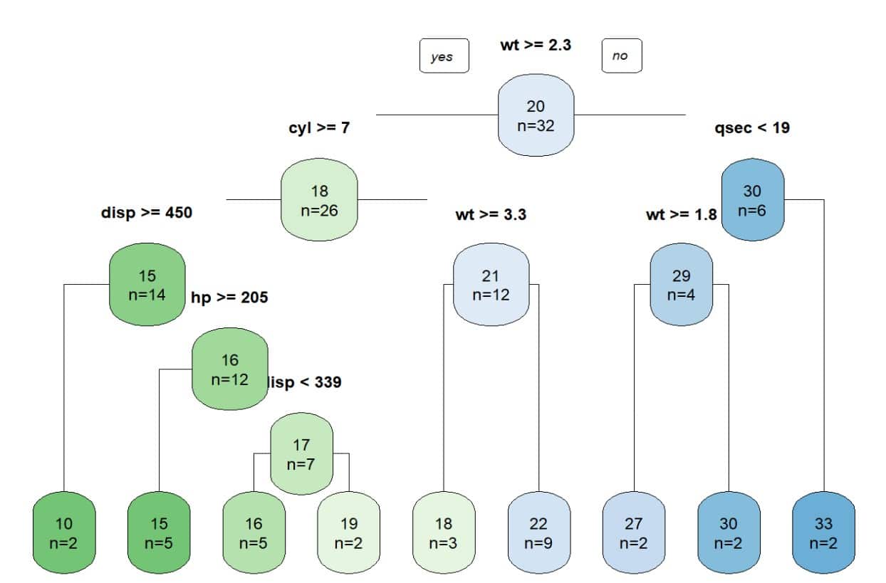
Although the recursive procedure that we have just seen can provide good predictions, it can sometimes lead to overfitting of the data and a more complex and difficult to interpret tree, like the one you see in the next figure.

In these cases, we have several alternatives. The first is to build, from the outset, a simpler tree. For example, we can begin to divide the space of predictor variables until we reach a predetermined number of nodes, cases per final node, or a certain value of the sum of squares of the residuals that we do not need to go below.

Another possibility is to build a very complex complete tree and proceed to trim some of its branches, considering all the sub-trees and their sums of squares. The problem could be very computationally infeasible.

A more practical option is to resort to a trick like the one used to estimate the lasso regression coefficients: penalize the least squares function by adding a factor that would be the product of the number of desired terminal nodes by a parameter called alpha, which would act as the balance between the complexity of the tree and its predictive capacity.

When α = 0, the tree we obtain is the complete one. However, when α increases, the least squares function is penalized and a tree with fewer branches is generated. We can generate several trees with successive values of α and choose the one that best weights, according to our criteria, the aspects of complexity and precision that interest us.

Decision trees for classification

Everything we have seen so far concerned decision trees designed to estimate or predict the value of a quantitative variable. In other words, we have talked about decision trees for regression. But trees can also serve as classification methods, which is the same as saying that they can estimate a qualitative response variable.

In these cases, the construction method follows a similar reasoning to that of regression trees, but has some differences, especially in the error function that we use to build the tree.

To show you an example of classification, I am going to use the “Pima.te” data set, from the R package MASS.

This data set contains a record of 332 pregnant women over 21 years of age who are evaluated for a diagnosis of gestational diabetes according to WHO criteria. In addition to the diagnosis of diabetes (yes/no), it contains information on the number of pregnancies, plasma glucose, systolic blood pressure, triceps fold, body mass index, history of diabetes and age.

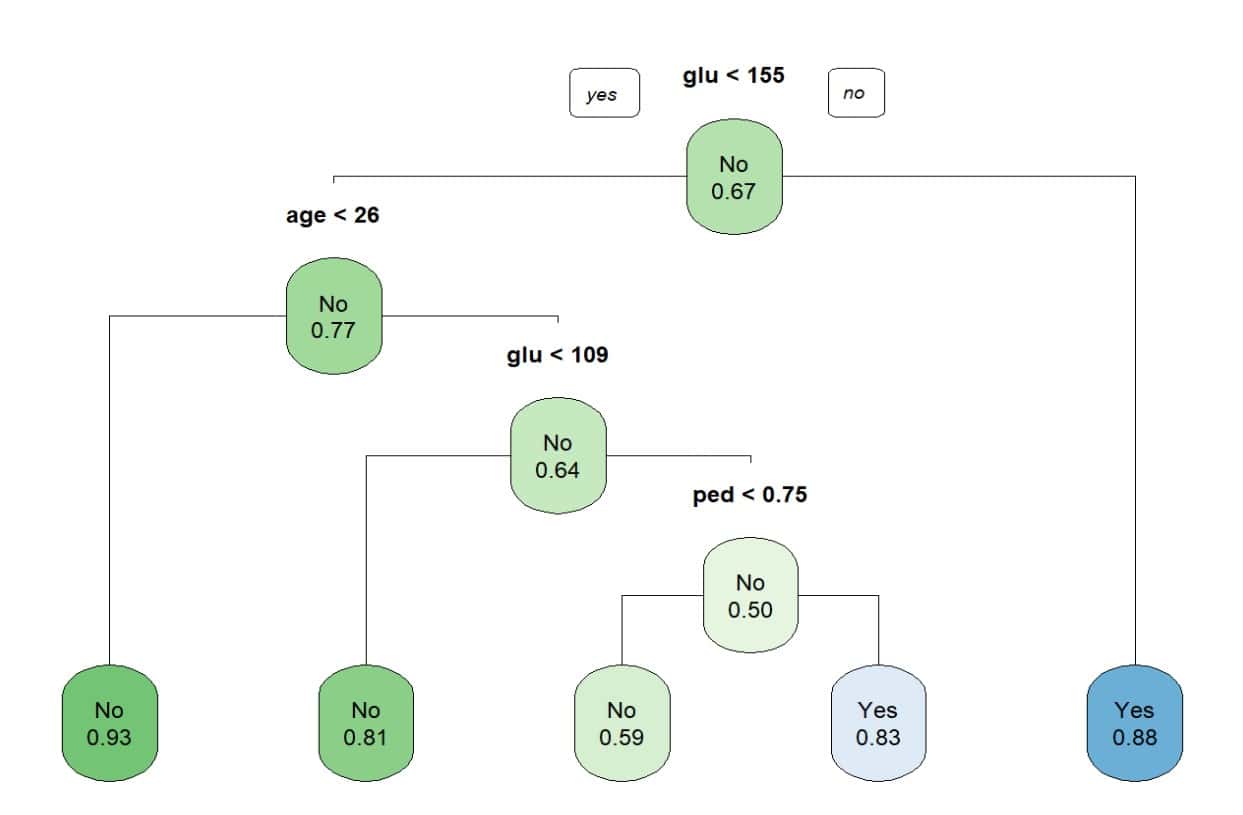
In this data set there are 109 diabetics and 223 non-diabetics. You can see the decision tree in figure 4.

Since it is a classification algorithm, in the terminal nodes we do not see the estimated value, as in the previous case, but rather the probability of belonging to the specified category. For example, a woman with a blood glucose level of less than 155 and age less than 26 years has a 93% probability of NOT being diabetic (or a 7% probability of being diabetic).

Building trees for classification

The mechanism is similar to the recursive steps that we have seen for regression trees, but the criterion of minimizing the sum of the squares of the residuals that we used before does not work in this case.

One possibility would be to calculate the percentage of classification errors, which would be the proportion of values in a region that do not belong to the majority category of that region. This method is relatively simple, but in practice it is not sensitive enough to produce trees with good predictive ability.

Instead, two indices that have been developed for this purpose are used: the Gini index and the entropy index. Let’s see what they consist of.

Gini index

The Gini index measures the total variance that exists between the different categories of the qualitative response variable. For this reason, its value tends to zero when the proportion of cases of a terminal node that belong to a given category increases. This is why the Gini index is considered a measure of the purity of the node.

For example, if we look at the first two nodes in the previous figure, the first (with 67% non-diabetics) is considered to be of lower purity than the second (77% non-diabetics). The lower the Gini index, the higher the proportion of observations of the same class in the node.

Entropy index

In this index, inspired by information theory, entropy refers to the measure of uncertainty or disorder in a data set. In this context, it is about determining how the data is divided between the different nodes of the tree, with the objective of maximizing the homogeneity of the classes within each node, which is the same as minimizing entropy.

If we think about it a little, it is practically the same thing that the Gini index tries to do, so it is not surprising that, in practice, both have a similar numerical value.

The three ways of quantifying the error can be used to construct the trees, although there are authors who prefer the Gini index or the entropy index for elaborating the tree and resort to the percentage of classification errors when it comes to trimming an already constructed tree.

We are leaving…

And with this we are going to leave gardening for today.

We have seen the system used by the decision tree algorithm to recursively divide the space of the predictor variables in order to estimate or predict the value of the target response variable, which can be both numerical (regression trees) or nominal (classification trees).

As many of you may have already thought, these types of predictions are the same that we can make with linear or logistic regression models (in reality, logistic regression is not a regression method, but rather a classification method). How do trees perform compared to the more classic methods we are more familiar with?

Well, as always, it will depend on the problem we are analysing. If we want to predict a numerical variable and our data fits well with a linear model, regression will work better than trees. However, if the data follow a more complex nonlinear relationship, we may improve our predictions by using decision trees.

Although trees have the undoubted advantage of their graphical interpretation and visualization, they do not usually achieve precision values as high as other regression or classification models. Furthermore, they are not very robust in the sense that small changes in the data can result in large variations in the trees we build.

Of course, all this can be substantially improved by using that old principle that says that there is strength in numbers. I am referring to the use of trees that employ aggregative resampling techniques (bagging), random forests, and other decision tree assembly methods. But that is another story…