Heterogeneity in meta-analysis.

The study of heterogeneity in meta-analysis is an essential part of its elaboration. Available methods are described.
Variety is good for many things. How boring the world would be if we were all the same! (especially if we all were like one that is now occurring to me). We like to go to different places, eating different meals, meet different people and have fun in different environments. But there’re things for which variety is a pain in the ass.
Think we have a set of clinical trials on the same topic and we want to perform a meta-analysis to obtain a global outcome. In this situation, we need as less variability as possible among studies if we’re going to combine them. Because, ladies and gentlemen, here prevails to be side by side but not eye to eye.
Heterogeneity in meta-analysis
Before thinking about combining the studies from a systematic review to perform a meta-analysis we should always carry out a preliminary asses of the heterogeneity of primary studies, which is just the measure of the variability that exists among the estimates that have been obtained in each of these studies.
First, we’ll investigate possible causes of heterogeneity, such us differences in treatment, variability among populations from different studies, and differences in trial designs.
Once we are convinced that studies seem to be homogeneous enough to try to combine them, we should try to measure this heterogeneity in an objective way. To do this, various gifted brains have created a series of statistics that contribute to our common jungle of acronyms and initials.
Q de Cochran
Until recently, the most famous of those initials was the Cochran’s Q, which has nothing to do either with James Bond or our friend Archie Cochrane. Its calculation takes into account the sum of the deviations between each of the results of primary studies and the global outcome (squared differences to avoid positives cancelling negatives), weighing each study according to their contribution to overall result. It looks awesome but actually, no big deal. Ultimately, it’s no more than an aristocratic relative of chi-square test. Indeed, Q follows a chi-square distribution with k-1 degrees of freedom (being k the number of primary studies). We calculate its value, look at the frequency distribution and estimate the probability that differences are not due to chance, in order to reject our null hypothesis (which assumes that observed differences among studies are due to chance). But, despite the appearances, Q has a number of weaknesses.
First, it’s a very conservative parameter and we must always keep in mind that lack of statistical significance is not always synonymous of absence of heterogeneity: as a matter of fact, we cannot reject the null hypothesis, so we have to know that when we approved it we are running the risk of committing a type II error and blunder. For this reason, some people propose to use a significance level of p < 0.1 instead of the standard p < 0.5. Another Q’s pitfall is that it doesn’t quantify the degree of heterogeneity and, of course, doesn’t explain the reasons that produce it. And, to top it off, Q loses power when the number of studies is small and doesn’t allow comparisons between different meta-analysis if they have different number of studies.
I2
This is why another statistic has been devised that is much more celebrated today: I2. This parameter provides an estimate of total variation among studies with respect to total variability or, put it another way, the proportion of variability actually due to heterogeneity for actual differences among the estimates compared with variability due to chance. It also looks impressive, but it’s actually an advantageous relative of the intraclass correlation coefficient.
Its value ranges from 0 to 100%, and we usually consider the limits of 25%, 50% and 75% as signs of low, moderate and high heterogeneity, respectively. I2 is not affected either by the effects units of measurement or the number of studies, so it allows comparisons between meta-analysis with different units of effect measurement or different number of studies.
If you read a study that provides Q and you want to calculate I2, or vice versa, you can use the following formula, being k the number of primary studies:
There’s a third parameter that is less known, but not less worthy of mention: H2. It measures the excess of Q value in respect of the value that we would expect to obtain if there were no heterogeneity. Thus, a value of 1 means no heterogeneity and its value increases as heterogeneity among studies does. But its real interest is that it allows calculating I2 confidence intervals.
Don’t worry about the calculations of Q, I2 and H2. Specific software is available to do that, such as RevMan or other modules that work with usual statistical programs.
And now I want to call your attention to one point: you must always remember that failure to prove heterogeneity does not always mean that studies are homogeneous. The problem is that null hypothesis assumes they are homogeneous and that differences that we observe are due to chance. If we can reject the null hypothesis we can ensure that there’s heterogeneity. But this doesn’t work the other way around: if we cannot reject it, it simply means that we cannot reject the existence of heterogeneity, but there is always a probability of making a type II error if we directly assume the studies are homogeneous.
Graphic methods
This is the reason why some people have devised a series of graphical methods to inspect the results and check if there is evidence of heterogeneity, no matter what numerical parameters say.
Galbraith’s graph
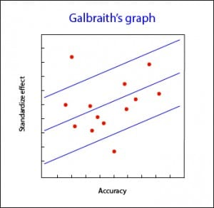
The most employed of them is, perhaps, the Galbraith’s plot, with can be used for both meta-analysis from trials or observational studies. This graph represents the accuracy of each study versus the standardize effects. It also shows the adjusted regression line and sets two confidence bands. The position of each study regarding the accuracy axis indicates its weighted contribution to overall results, while its location outside the confidence bands indicates its contribution to heterogeneity.
Galbraith’s graph can also be useful for detecting sources of heterogeneity, since studies can be labeled according to different variables and see how they contribute to the overall heterogeneity.
L’Abbé’s graph
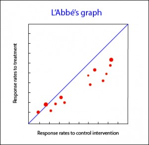
Another available tool you can use for meta-analysis of clinical trials is L’Abbé plot. It represents response rates to treatment versus response rates in control group, plotting the studies to both sides of the diagonal. Above that line are studies with positive treatment outcome, while below are studies with an outcome favorable to control intervention. The studies usually are plotted with an area proportional to its accuracy, and its dispersion indicates heterogeneity. Sometimes, L’Abbé graph provides additional information. For example, in the accompanying graph you can see that studies in low-risk areas are located mainly below the diagonal. On the other hand, high-risk studies are mainly located in areas of positive treatment outcome. This distribution, as well as being suggestive of heterogeneity, may suggest that efficacy of treatments depends on the level of risk or, put another way, we have an effect modifying variable in our study.
Having examined the homogeneity of primary studies we can come to the grim conclusion that heterogeneity reigns supreme in our situation. Can we do something to manage it?. Sure, we can. We can always not to combine the studies, or combine them despite heterogeneity and obtain a summary result but, in that case, we should also calculate any measure of variability among studies and yet we could not be sure of our results.
Another possibility is to do a stratified analysis according to the variable that causes heterogeneity, provided that we are able to identify it. For this we can do a sensitivity analysis, repeating calculations once removing one by one each of the subgroups and checking how it influences the overall result. The problem is that this approach ignores the final purpose of any meta-analysis, which is none than obtaining an overall value of homogeneous studies.
Meta-regression
Finally, the brainiest on these issues can use meta-regression. This technique is similar to multivariate regression models in which the characteristics of the studies are used as explanatory variables, and effect’s variable or some measure of deviation of each study with respect to global result are used as dependent variable. Also, it should be done a weighting according to the contribution of each study to the overall result and try not to score too much coefficients to the regression model if the number of primary studies is not large. I wouldn’t advise you to do a meta-regression at home if it is not accompanied by seniors.
We’re leaving…
And we’re done for now. Congratulations to which have endured so far. I apologize for the drag I have released, but heterogeneity has something in it. And it is not only important to decide whether or not to combine the studies, but it is also very important to decide what data analysis model we have to use. But that’s another story…


