Regression model diagnostics.

We live in a crazy world, always running from here to there and always with a thousand things in mind. Thus, it is not uncommon for us to leave many of our tasks half finished.
This will be of little importance in some occasions, but there will be others in which leaving things half done will make the other half we have done useless.
And this is precisely what happens when we apply this sloppiness to our topic of today: we do an experiment, we calculate a regression line and we just start applying it, forgetting to make a regression model diagnostics.
In these cases, leaving things half done may have the consequence that we apply to our population a predictive model that, in reality, may not be valid.
Raising the problem
We already saw in a previous post how to build a simple linear regression model. As we already know, simple linear regression allows us to estimate what the value of a dependent variable will be based on the value taken by a second variable, which will be the independent one, provided that there is a linear relationship between the two variables.
We also saw in an example how a regression model could allow us to estimate what the height of a tree would be if we only know the volume of the trunk, even if we did not have any tree with that volume available.
No wonder, then, that the prediction capabilities of regression models are widely used in biomedical research. And that’s fine, but the problem is that, the vast majority of the time, authors who use regression models to communicate their studies’ results forget about the validation and diagnostics of the regression model.
And at this point, some may wonder: do regression models have to be validated? If we already have the coefficients of the model, do we have to do something else?
Well, yes, it is not enough to obtain the coefficients of the line and start making predictions. To be sure that the model is valid, a series of assumptions must be checked. This process is known as the validation and regression model diagnostics.
Validation of a regression model
We must never forget that we usually deal with samples, but what we really want is to make inferences about the population from which the sample comes, which we cannot access in its entirety.
Once we calculate the coefficients of the regression line using, for example, the least squared method, and we see that their valuea are different from zero, we must ask ourselves if it is possible that in the population that value are zero and that the values that we have found in our sample are due to random fluctuations.
And how can we know this? Very easy, we will make a hypothesis contrast for the two coefficients of the line with the null hypothesis that the coefficients values are, effectively, zero:
H0 : β0 = 0 y H0 : β1 = 0
If we can reject both null hypotheses, we can apply the regression line that we have obtained to our population.
If we cannot reject H0 for β0, the constant (interceptor) of the model will not be valid. We can still apply the lineal equation, but assuming it originates from the coordinate axis. But if we have the misfortune of not being able to reject the null hypothesis for the slope (or for neither of the two coefficients), we will not be able to apply the model to the population: the independent variable will not allow us to predict the value of the dependent variable.
This hypothesis contrast can be done in two ways:
- If we divide each coefficient by its standard error, we will obtain a statistic that follows a Student’s t distribution with n-2 degrees of freedom. We can calculate the p-value associated with that value and solve the hypothesis contrast by rejecting the null hypothesis if p<0.05.
- A slightly more complex way is to base this hypothesis contrast on an analysis of variance (ANOVA). This method considers that the variability of the dependent variable is decomposed into two terms: one explained by the independent variable and the other not assigned to any source and which is considered unexplained (random).
It is possible to obtain the estimate of the variance of the error of both components, explained and unexplained. If the variation due to the independent variable does not exceed that of chance, the ratio of explained / unexplained will have a value close to one. Otherwise, it will move away from unity, the more the better predictions of the dependent variable provided by the independent variable.
When the slope (the coefficient β1) is equal to zero (under the assumption of the null hypothesis), this quotient follows a Snedecor’s F distribution with 1 and n-2 degrees of freedom. As with the previous method, we can calculate the p-value associated with the value of F and reject the null hypothesis if p <0.05.
Let’s see an example
We are going to try to understand a little better what we have just explained by using a practical example. To do this, we are going to use the statistical program R and one of its data sets, “trees”, which collects the circumference, volume and height of 31 observations on trees.
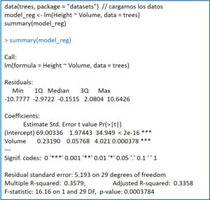
If you look closely, the program shows the point estimate of the coefficients together with their standard errors. This is accompanied by the values of the t statistic with their statistical significance. In both cases, the value of p <0.05, so we reject the null hypothesis for the two coefficients of the equation of the line. In other words, both coefficients are statistically significant.
Next, R provides us with a series of data (the standard deviation of the residuals, the square of the multiple correlation coefficient or coefficient of determination and its adjusted value) among which is the F’s contrast to validate the model. There are no surprises, p is less than 0.05, so we can reject the null hypothesis: the coefficient β1 is statistically significant and the independent variable allows predicting the values of the dependent variable.
Regression model diagnostics
Everything we have seen so far is usually provided by statistical programs when we ask for the regression model. But we cannot leave the task half done. Once we have verified that the coefficients are significant, we can ensure that a series of necessary assumptions are met for the model to be valid.
These assumptions are four: linearity, homoscedasticity, normality and independence. Here, even if we use a statistics program, we will have to work a Little hard to verify these assumptions and make a correct diagnostics of the regression model.
Linearity assumption
As we have already commented, the relationship between the dependent and independent variables must be linear. This can be seen with something as simple as scatter plot, which shows us what the relationship looks like in the range of observed values of the independent variable.
If we see that the relationship is not linear and we are very determined to use a linear regression model, we can try to make a transformation of the variables and see if the points are already distributed, more or less, along a line.
A numerical method that enables the assumption of linearity to be tested is Ramsey’s RESET test. This test checks whether it is necessary to introduce quadratic or cubic terms so that the systematic patterns in the residuals disappear. Let’s see what this means.
The residual is the difference between a real value of the dependent variable observed in the experiment and the value estimated by the regression model. In the previous image that shows the result of the summary() function of R we can see the distribution of the residuals.
For the model to be correct, the median must be close to zero and the absolute values of the residuals must be uniformly distributed among the quartiles (similar between maximum and minimum and between first and third quartiles). In other words, this means that the residuals, if the model is correct, follow a normal distribution whose mean is zero.
If we see that this is not the case, the residuals will be systematically biased and the model will be incorrectly specified. Logically, if the model is not linear, this bias of the residuals could be corrected by introducing a quadratic or cubic term into the equation of the line. Of course, then, it would no longer be a linear regression nor the equation of a line.
The null hypothesis of the Ramsey’s test says that the terms quadratic, cubic, or both are equal to zero (they can be tested together or separately). If we cannot reject the null hypothesis, the model is assumed to be correctly specified. Otherwise, if we reject the null hypothesis, the model will have specification errors and will have to be revised.
Homoscedasticity assumption
We have already commented: the residuals must be distributed homogeneously for all the values of the prediction variable.
This can be verified in a simple way with a scatter plot that represents, on the abscissa axis, the estimates of the dependent variable for the different values of the independent variable and, on the coordinate axis, the corresponding residuals. The homoscedasticity assumption will be accepted if the residuals are randomly distributed, in which case we will see a cloud of points in a similar way throughout the range of the observations of the independent variable.
We also have numerical methods to test the assumption of homoscedasticity, such as the Breusch-Pagan-Godfrey test, whose null hypothesis states that this assumption is satisfied.
Assumption of normality
We have also said it already: the residues must be distributed in a normal way.
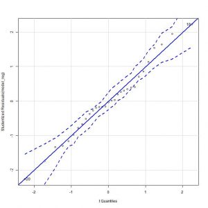
A simple way to check it would be to represent the graph of theoretical quantiles of the residuals, in which we should see their distribution along the diagonal of the graph.
We can also use a numerical method, such as the Kolmogorov-Smirnov’s test or the Shapiro-Wilk’s test.
Independence assumption
Finally, the residuals must be independent of each other and there have to be no correlation among them.
This can be contrasted by carrying out the Durbin-Watson’s test, whose null hypothesis assumes precisely that the residuals are independent.
Let’s go back to our example
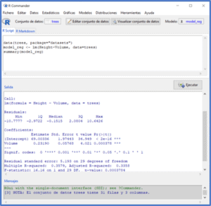
For those of you who don’t know R very well, I leave you on the first screen the previous steps to load the data and calculate the regression model.
Let’s start with the diagnosis of the model.
To check if the assumption of linearity is fulfilled, we start by drawing the scatter plot with the two variables (menu options Graphs-> Scatter plot). If we look at the graph, we see that the points are distributed, more or less, along a line in an upward direction to the right.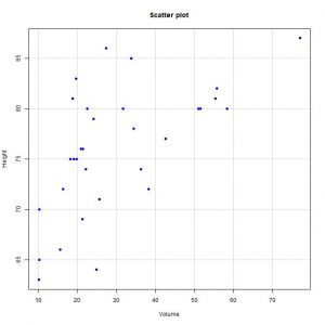
If we want to do the numerical method, we select the menu option Models-> Numerical diagnostics-> Non-linearity RESET test. R gives us a RESET value = 2.52, with a p = 0.09. As p> 0.05, we cannot reject the null hypothesis that the model is linear, thereby corroborating the impression we obtained with the graphic method.
Let’s go with homoscedasticity. For the graphical method we resort to the menu option Models-> Graphs-> Basic diagnostic graphs. The program provides us with 4 graphs, but now we will only look at the first one, which represents the values predicted by the model of the dependent variable against the residuals.
As can be seen, the dispersion of the points is much greater for the lower values of the dependent variable, so I would not be very calm about whether the homoscedasticity assumption is fulfilled. The points should be distributed homogeneously over the entire range of values of the dependent variable.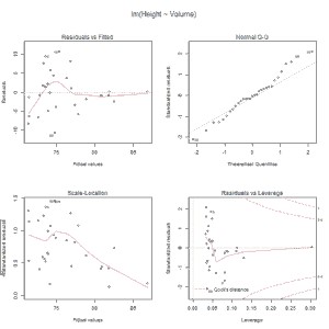
Let’s see what the numerical method says. We select the menu option Models-> Numerical diagnoses-> Breusch-Pagan test for heteroscedasticity. The value of the BP statistic that R gives us is 2.76, with a p-value = 0.09. Since p> 0.05, we cannot reject the null hypothesis, so we assume that the homoscedasticity assumption holds.
We went on to check the normality of the residuals. For the graphical diagnostic method, we select the menu option Graphs-> Graph of comparison of quantiles. This time there is no doubt, it seems that the points are distributed along the diagonal.
Finally, let’s check the independence assumption.
Consequently, we cannot reject the null hypothesis that the residuals are independent, thus fulfilling the last condition to consider the model as valid.
We are leaving…
And here we are going to leave it for today. Seeing how laborious this whole procedure is, one can fall into the temptation to forgive and even understand the authors who hide the diagnostics of their regression models from us. But this excuse is not valid: statistical programs do it refrained from making the least effort.
Do not think that with everything we have explained we have done everything we should before applying a simple linear regression model with confidence.
For example, it would not hurt to assess whether there are influential observations that may have a greater weight in the formulation of the model. Or if there are extreme values (outliers) that can distort the estimate of the slope of the regression line. But that is another story…
