Sensitivity and specificity.

The concepts of sensitivity and specificity, predictive values and likelihood ratios are described, as well as the use of ROC curves.
The world of medicine is a world of uncertainty. We can never be sure of anything at 100%, however obvious it may seem a diagnosis, but we cannot beat right and left with ultramodern diagnostics techniques or treatments (that are never safe) when making the decisions that continually haunt us in our daily practice.
That’s why we are always immersed in a world of probabilities, where the certainties are almost as rare as the so-called common sense which, as almost everyone knows, is the least common of the senses.
Imagine you are in the clinic and a patient comes because he has been kicked in the ass, pretty strong, though. As good doctor as we are, we ask that of what’s wrong?, since when?, and what do you attribute it to? And we proceed to a complete physical examination, discovering with horror that he has a hematoma on the right buttock.
Different approaches for a differential diagnosis
Here, my friends, the diagnostic possibilities are numerous, so the first thing we do is a comprehensive differential diagnosis. To do this, we can take four different approaches. The first is the possibilistic approach, listing all possible diagnoses and try to rule them all simultaneously applying the relevant diagnostic tests.
The second is the probabilistic approach, sorting diagnostics by relative chance and then acting accordingly. It seems a posttraumatic hematoma (known as the kick in the ass syndrome), but someone might think that the kick has not been so strong, so maybe the poor patient has a bleeding disorder or a blood dyscrasia with secondary thrombocytopenia or even an atypical inflammatory bowel disease with extraintestinal manifestations and gluteal vascular fragility.
We could also use a prognostic approach and try to show or rule out possible diagnostics with worst prognosis, so the diagnosis of the kicked in the ass syndrome lose interest and we were going to rule out chronic leukemia. Finally, a pragmatic approach could be used, with particular interest in first finding diagnostics that have a more effective treatment (the kick will be, one more time, the number one).
It seems that the right thing is to use a judicious combination of pragmatic, probabilistic and prognostic approaches. In our case we will investigate if the intensity of injury justifies the magnitude of bruising and, in that case, we would indicate some hot towels and we would refrain from further diagnostic tests. And this example may seems to be bullshit, but I can assure you I know people who make the complete list and order the diagnostic tests when there are any symptoms, regardless of expenses or risks.
And, besides, one that I could think of, could assess the possibility of performing a more exotic diagnostic test that I cannot imagine, so the patient would be grateful if the diagnosis doesn’t require to make a forced anal sphincterotomy. And that is so because, as we have already said, the waiting list to get some common sense exceeds in many times the surgical waiting list.
The two thresholds
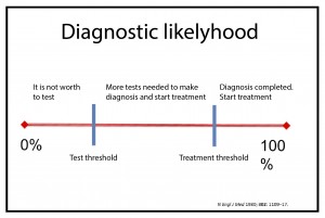 Now imagine another patient with a symptom complex less stupid and absurd than the previous example. For instance, let’s think about a child with symptoms of celiac disease. Before we make any diagnostic test, our patient already has a probability of suffering the disease.
his probability will be conditioned by the prevalence of the disease in the population from which she proceeds and is called the pretest probability. This probability will stand somewhere between two thresholds: the diagnostic threshold and the therapeutic threshold.
The usual thing is that the pre-test probability of our patient does not allow us to rule out the disease with reasonable certainty (it would have to be very low, below the diagnostic threshold) or to confirm it with sufficient security to start the treatment (it would have to be above the therapeutic threshold).
We’ll then make the indicated diagnostic test, getting a new probability of disease depending on the result of the test, the so-called post-test probability. If this probability is high enough to make a diagnosis and initiate treatment, we’ll have crossed our first threshold, the therapeutic one. There will be no need for additional tests, as we will have enough certainty to confirm the diagnosis and treat the patient, always within a range of uncertainty.
And what determines our treatment threshold? Well, there are several factors involved. The greater the risk, cost or adverse effects of the treatment in question, the higher the threshold that we will demand to be treated. In the other hand, as much more serious is the possibility of omitting the diagnosis, the lower the therapeutic threshold that we’ll accept.
But it may be that the post-test probability is so low that allows us to rule out the disease with reasonable assurance. We shall then have crossed our second threshold, the diagnostic one, also called the no-test threshold. Clearly, in this situation, it is not indicated further diagnostic tests and, of course, starting treatment.
However, very often changing pretest to post-test probability still leaves us in no man’s land, without achieving any of the two thresholds, so we will have to perform additional tests until we reach one of the two limits.
And this is our everyday need: to know the post-test probability of our patients to know if we discard or confirm the diagnosis, if we leave the patient alone or we lash her out with our treatments. And this is so because the simplistic approach that a patient is sick if the diagnostic test is positive and healthy if it is negative is totally wrong, even if it is the general belief among those who indicate the tests. We will have to look, then, for some parameter that tells us how useful a specific diagnostic test can be to serve the purpose we need: to know the probability that the patient suffers the disease.
The guard’s dilemma
And this reminds me of the enormous problem that a brother-in-law asked me about the other day. The poor man is very concerned with a dilemma that has arisen. The thing is that he’s going to start a small business and he wants to hire a security guard to stay at the entrance door and watch for those who take something without paying for it.
And the problem is that there’re two candidates and he doesn’t know who of the two to choose. One of them stops nearly everyone, so no burglar escapes. Of course, many honest people are offended when they are asked to open their bags before leaving and so next time they will buy elsewhere. The other guard is the opposite: he stops almost anyone but the one he spots certainly brings something stolen. He offends few honest people, but too many grabbers escape. A difficult decision…
Why my brother-in-law comes to me with this story? Because he knows that I daily face with similar dilemmas every time I have to choose a diagnostic test to know if a patient is sick and I have to treat her. We have already said that the positivity of a test does not assure us the diagnosis, just as the bad looking of a client does not ensure that the poor man has robbed us.
Let’s see it with an example. When we want to know the utility of a diagnostic test, we usually compare its results with those of a reference or gold standard, which is a test that, ideally, is always positive in sick patients and negative in healthy people. Now let’s suppose that I perform a study in my hospital office with a new diagnostic test to detect a certain disease and I get the results from the attached table (the patients are those who have the positive reference test and the healthy ones, the negative).
Sensitivity and specificity
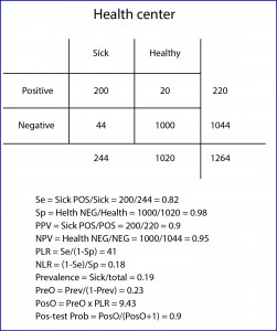 Let’s start with the easy part. We have 1598 subjects, 520 out of them sick and 1078 healthy. The test gives us 446 positive results, 428 true (TP) and 18 false (FP). It also gives us 1152 negatives, 1060 true (TN) and 92 false (FN). The first we can determine is the ability of the test to distinguish between healthy and sick, which leads me to introduce the first two concepts: sensitivity (Se) and specificity (Sp).
Se is the likelihood that the test correctly classifies a patient or, in other words, the probability that a patient gets a positive result. It’s calculated dividing TP by the number of sick. In our case it equals 0.82 (if you prefer to use percentages you have to multiply by 100). Moreover, Sp is the likelihood that the test correctly classifies a healthy or, put another way, the probability that a healthy gets a negative result. It’s calculated dividing TN by the number of healthy. In our example, it equals 0.98.
Someone may think that we have assessed the value of the new test, but we have just begun to do it. And this is because with Se and Sp we somehow measure the ability of the test to discriminate between healthy and sick, but what we really need to know is the probability that an individual with a positive results being sick and, although it may seem to be similar concepts, they are actually quite different.
The probability of a positive of being sick is known as the positive predictive value (PPV) and is calculated dividing the number of patients with a positive test by the total number of positives. In our case it is 0.96. This means that a positive has a 96% chance of being sick. Moreover, the probability of a negative of being healthy is expressed by the negative predictive value (NPV), with is the quotient of healthy with a negative test by the total number of negatives.
In our example it equals 0.92 (an individual with a negative result has 92% chance of being healthy). This is already looking more like what we said at the beginning that we needed: the post-test probability that the patient is really sick.
Predictive values
And from now on is when neurons begin to be overheated. It turns out that Se and Sp are two intrinsic characteristics of the diagnostic test. Their results will be the same whenever we use the test in similar conditions, regardless of the subjects of the test. But this is not so with the predictive values, which vary depending on the prevalence of the disease in the population in which we test. This means that the probability of a positive of being sick depends on how common or rare the disease in the population is. Yes, you read this right: the same positive test expresses different risk of being sick, and for unbelievers, I’ll put another example.
 Suppose that this same study is repeated by one of my colleagues who works at a community health center, where population is proportionally healthier than at my hospital (logical, they have not suffered the hospital yet). If you check the results in the table and bring you the trouble to calculate it, you may come up with a Se of 0.82 and a Sp of 0.98, the same that I came up with in my practice. However, if you calculate the predictive values, you will see that the PPV equals 0.9 and the NPV 0.95. And this is so because the prevalence of the disease (sick divided by total) is different in the two populations: 0.32 at my practice vs 0.19 at the health center.
That is, in cases of highest prevalence a positive value is more valuable to confirm the diagnosis of disease, but a negative is less reliable to rule it out. And conversely, if the disease is very rare a negative result will reasonably rule out disease but a positive will be less reliable at the time to confirm it.
We see that, as almost always happen in medicine, we are moving on the shaking ground of probability, since all (absolutely all) diagnostic tests are imperfect and make mistakes when classifying healthy and sick. So when is a diagnostic test worth of using it? If you think about it, any particular subject has a probability of being sick even before performing the test (the prevalence of disease in her population) and we’re only interested in using diagnostic tests if that increase this likelihood enough to justify the initiation of the appropriate treatment (otherwise we would have to do another test to reach the threshold level of probability to justify treatment).
Likelihood ratios
And here is when this issue begins to be a little unfriendly. The positive likelihood ratio (PLR), indicates how much more probable is to get a positive with a sick than with a healthy subject. The proportion of positive in sick patients is represented by Se. The proportion of positives in healthy are the FP, which would be those healthy without a negative result or, what is the same, 1-Sp. Thus, PLR = Se / (1 – Sp). In our case (hospital) it equals 41 (the same value no matter we use percentages for Se and Sp). This can be interpreted as it is 41 times more likely to get a positive with a sick than with a healthy.
It’s also possible to calculate NLR (negative), which expresses how much likely is to find a negative in a sick than in a healthy. Negative patients are those who don’t test positive (1-Se) and negative healthy are the same as the TN (the test’s Sp). So, NLR = (1 – Se) / Sp. In our example, 0.18.
A ratio of 1 indicates that the result of the test doesn’t change the likelihood of being sick. If it’s greater than 1 the probability is increased and, if less than 1, decreased. This is the parameter used to determine the diagnostic power of the test. Values > 10 (or > 0.01) indicates that it’s a very powerful test that supports (or contradict) the diagnosis; values from 5-10 (or 0.1-0.2) indicates low power of the test to support (or disprove) the diagnosis; 2-5 (or 0.2-05) indicates that the contribution of the test is questionable; and, finally, 1-2 (0.5-1) indicates that the test has not diagnostic value.
Postest probbility and Fagan’s nomogram
The likelihood ratio does not express a direct probability, but it helps us to calculate the probabilities of being sick before and after testing positive by means of the Bayes’ rule, which says that the posttest odds is equal to the product of the pretest odds by the likelihood ratio. To transform the prevalence into pre-test odds we use the formula odds = p / (1-p). In our case, it would be 0.47.
Now we can calculate the post-test odds (PosO) by multiplying the pretest odds by the likelihood ratio. In our case, the positive post-test odds value is 19.27. And finally, we transform the post-test odds into post-test probability using the formula p = odds / (odds + 1). In our example it values 0.95, which means that if our test is positive the probability of being sick goes from 0.32 (the pre-test probability) to 0.95 (post-test probability).
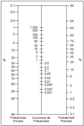 If there’s still anyone reading at this point, I’ll say that we don’t need all this gibberish to get post-test probability. There are multiple websites with online calculators for all these parameters from the initial 2 by 2 table with a minimum effort. I addition, the post-test probability can be easily calculated using a Fagan’s nomogram (see attached figure). This graph represents in three vertical lines from left to right the pre-test probability (it is represented inverted), the likelihood ratios and the resulting post-test probability.
To calculate the post-test probability after a positive result, we draw a line from the prevalence (pre-test probability) to the PLR and extend it to the post-test probability axis. Similarly, in order to calculate post-test probability after a negative result, we would extend the line between prevalence and the value of the NLR.
In this way, with this tool we can directly calculate the post-test probability by knowing the likelihood ratios and the prevalence. In addition, we can use it in populations with different prevalence, simply by modifying the origin of the line in the axis of pre-test probability.
So far we have defined the parameters that help us to quantify the power of a diagnostic test and we have seen the limitations of sensitivity, specificity and predictive values and how the most useful in a general way are the likelihood ratios. But, you will ask, what is a good test?, is it a sensitive one?, a specific?, both?
Here we are going to return to the guard’s dilemma that has arisen to my poor brother-in-law, because we have left him abandoned and we have not answered yet which of the two guards we recommend him to hire, the one who ask almost everyone to open their bags and so offending many honest people, or the one who almost never stops honest people but, stopping almost anyone, many thieves get away.
The resolution of the dilemma
And what do you think is the better choice? The simple answer is: it depends. Those of you who are still awake by now will have noticed that the first guard (the one who checks many people) is the sensitive one while the second is the specific one. What is better for us, the sensitive or the specific guard? It depends, for example, on where our shop is located. If your shop is located in a heeled neighborhood the first guard won’t be the best choice because, in fact, few people will be stealers and we’ll prefer not to offend our customers so they don’t fly away.
But if our shop is located in front of the Cave of Ali Baba we’ll be more interested in detecting the maximum number of clients carrying stolen stuff. Also, it can depend on what we sell in the store. If we have a flea market we can hire the specific guard although someone can escape (at the end of the day, we’ll lose a few amount of money). But if we sell diamonds we’ll want no thieve to escape and we’ll hire the sensitive guard (we’ll rather bother someone honest than allows anybody escaping with a diamond).
The same happens in medicine with the choice of diagnostic tests: we have to decide in each case whether we are more interested in being sensitive or specific, because diagnostic tests not always have a high sensitivity (Se) and specificity (Sp).
In general, a sensitive test is preferred when the inconveniences of a false positive (FP) are smaller than those of a false negative (FN). For example, suppose that we’re going to vaccinate a group of patients and we know that the vaccine is deadly in those with a particular metabolic error. It’s clear that our interest is that no patient be undiagnosed (to avoid FN), but nothing happens if we wrongly label a healthy as having a metabolic error (FP): it’s preferable not to vaccinate a healthy thinking that it has a metabolopathy (although it hasn’t) that to kill a patient with our vaccine supposing he was healthy.
Another less dramatic example: in the midst of an epidemic our interest will be to be very sensitive and isolate the largest number of patients. The problem here if for the unfortunate healthy who test positive (FP) and get isolated with the rest of sick people. No doubt we’d do him a disservice with the maneuver. Of course, we could do to all the positives to the first test a second confirmatory one that is very specific in order to avoid bad consequences to FP people.
On the other hand, a specific test is preferred when it is better to have a FN than a FP, as when we want to be sure that someone is actually sick. Imagine that a test positive result implies a surgical treatment: we’ll have to be quite sure about the diagnostic so we don’t operate any healthy people.
Another example is a disease whose diagnosis can be very traumatic for the patient or that is almost incurable or that has no treatment. Here we´ll prefer specificity to not to give any unnecessary annoyance to a healthy. Conversely, if the disease is serious but treatable we´ll probably prefer a sensitive test.
ROC curves
So far we have talked about tests with a dichotomous result: positive or negative. But, what happens when the result is quantitative? Let’s imagine that we measure fasting blood glucose. We must decide to what level of glycemia we consider normal and above which one will seem pathological. And this is a crucial decision, because Se and Sp will depend on the cutoff point we choose.
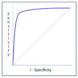 To help us to choose we have the receiver operating characteristic, known worldwide as the ROC curve. We represent in coordinates (y axis) the Se and in abscissas the complementary Sp (1-Sp) and draw a curve in which each point represents the probability that the test correctly classifies a healthy-sick couple taken at random. The diagonal of the graph would represent the “curve” if the test had no ability to discriminate healthy from sick patients.
As you can see in the figure, the curve usually has a segment of steep slope where the Se increases rapidly without hardly changing the Sp: if we move up we can increase Se without practically increasing FP. But there comes a time when we get to the flat part. If we continue to move to the right, there will be a point from which the Se will no longer increase, but will begin to increase FP. If we are interested in a sensitive test, we will stay in the first part of the curve.
If we want specificity we will have to go further to the right. And, finally, if we do not have a predilection for either of the two (we are equally concerned with obtaining FP than FN), the best cutoff point will be the one closest to the upper left corner. For this, some use the so-called Youden’s index, which optimizes the two parameters to the maximum and is calculated by adding Se and Sp and subtracting 1. The higher the index, the fewer patients misclassified by the diagnostic test.
A parameter of interest is the area under the curve (AUC), which represents the probability that the diagnostic test correctly classifies the patient who is being tested (see attached figure). An ideal test with Se and Sp of 100% has an area under the curve of 1: it always hits. In clinical practice, a test whose ROC curve has an AUC> 0.9 is considered very accurate, between 0.7-0.9 of moderate accuracy and between 0.5-0.7 of low accuracy.
On the diagonal, the AUC is equal to 0.5 and it indicates that it does not matter if the test is done by throwing a coin in the air to decide if the patient is sick or not. Values below 0.5 indicate that the test is even worse than chance, since it will systematically classify patients as healthy and vice versa.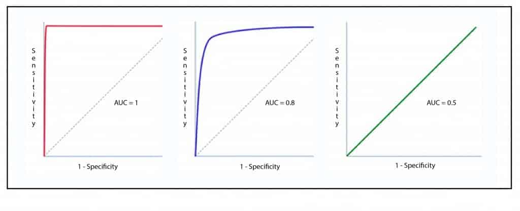
We’re leaving…
Curious these ROC curves, aren`t they? Its usefulness is not limited to the assessment of the goodness of diagnostic tests with quantitative results. The ROC curves also serve to determine the goodness of fit of a logistic regression model to predict dichotomous outcomes, but that is another story…
