Linear correlation.

We already know about the relationship between variables. Who can doubt that smoking kills or that TV dries our brain?. The issue is that we have to try to quantify these relationships in an objective way because, otherwise, here will always be someone who can doubt them. To do this, we’ll have to use some parameter which studies if our variables change in a related way.

When the two are dichotomous variables the solution is simple: we can use the odds ratio. Regarding TV and brain damage, we could use it to calculate whether it is really more likely to have dry brains watching too much TV (although I’d not waste time). But what happens if the two variables are continuous?. We cannot use then the odds ratio and we have to use other tools. Let’s see an example.

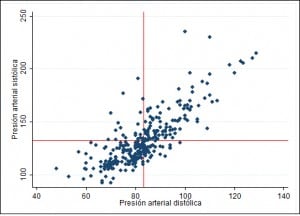
Suppose I take blood pressure to a sample of 300 people and represent the values of systolic and diastolic pressure, as I show in the first scatterplot. At a glance, you realize that it smells a rat. If you look carefully, high systolic pressure is usually associated with high diastolic values and, conversely, low values of systolic are associated with low diastolic values. I would say that they vary similarly: higher values of one with higher of the other, and vice versa. For a better view, look at the following two graphs.

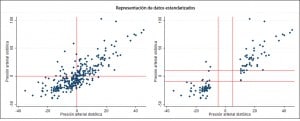
Standardized pressure values (each value minus the mean) are shown in the first graph. We see that most of the points are in the lower left and upper right quadrants. You can still see it better in the second chart, in which I’ve omitted values between systolic ± 10 mmHg and diastolic ± 5 mmHg around zero, which would be the standardized means. Let’s see if we can quantify this somehow.

Remember that the variance measured how varied the values of a distribution respect to the mean. We subtract the mean to each value, the result is squared so it’s always positive (to avoid that positive and negative differences cancelled each other), all these differences are added and the sum is divided by the sample size (in reality, the sample size minus one, and do not ask why, only mathematicians know why). You know that the square root of the variance is the standard deviation, the queen of the measures of dispersion.

Covariance

Well, with a couple of variables we can do a similar thing. We calculate, for every couple, the differences of every variable with their means and multiply these differences (the equivalent of squaring the difference we did with the variance). Finally, we add all these products and divided the result by the sample size minus one, thus obtaining this version of the couples’s variance which is called, how could it be otherwise, covariance.

And what tells us the value of covariance?. Well, not much, as it will depend on the magnitudes of the variables, which can be different depending on what we are talking about. To circumvent this little problem we use a very handy solution in such situations: standardize.

Pearson’s linear correlation coefficient

Thus, we divide the differences from the mean by their standard deviations, obtaining the world famous linear correlation coefficient of Pearson.

It’s good to know that, actually, Pearson only made the initial development of the above mentioned coefficient and that the real father of the creature was Francis Galton. The poor man spent all his life trying to do something important because he was jealous of his cousin, much more famous, one Charles Darwin, which I think he wrote about a species that eat each other and saying that the secret is to procreate as much as possible to survive.

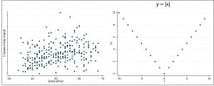
Pearson’s correlation coefficient, r for friends, can have any value from -1 to 1. When set to zero means that the variables are uncorrelated, but do not confuse this with the fact that whether they are or not independent; as the tittle of this post says, the Pearson’s coefficient relationship does not compromise variables to anything serious. Correlation and independence have nothing to do with each other, they are different concepts. If you look at the two graphs of the example you’ll see that r equals zero in both. However, although the variables in the first one are independent, this is not true for the second, which represents the function y = |x|.

If r is greater than zero it means that the correlation is positive, so that the two variables vary in the same sense: when one increases, so does the other and, conversely, when the second decreases so decreases the other one. It is said that this positive correlation is perfect when r is 1. On the other hand, when r is negative, it means that the variables vary in the opposite way: when one increases the other decreases, and vice versa. Again, the negative correlation is perfect when r is -1.

Linear correlation doesn’t imply causality

It is crucial to understand that correlation doesn’t always mean causality. As Stephen J. Gould said in his book “The false measure of man” to take this fact is one of the two or three most serious and frequent errors of human reasoning. And it must be true because, even though I searched, I have not found any cousin to which he wanted to shadow, which makes me think he said it because he was convinced. So now you know, even though when there’s causality there’s correlation, the opposite is not always true.

Situations needed to apply linear correlation

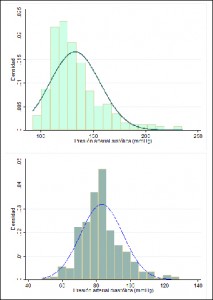
Another mistake we can make is to use this coefficient without making a series of preflight checks. The first is that the correlation between the two variables must be linear. This is easy to check by plotting the points and seeing that does not look like a parabola, hyperbole or any other curved shape. The second is that at least one of the variables should follow a normal distribution of frequencies. For this we can use statistical tests such as Kolmogorov-Smirnov’s or Shapiro-Wilks’, but often it is enough with representing histograms with frequency curves and see if they fit the normal.

In our case, diastolic may fit a normal curve, but I’d not hold my breath for the systolic. The form of the cloud of point in the scatter plot gives us another clue: elliptical or rugby ball shape indicates that the variables probably follow a normal distribution. Finally, the third test is to ensure that samples are random. In addition, we can only use r within the range of data. If we extrapolated outside this range, we’d make an error.

A final warning: do not confuse correlation with regression. Correlation investigates the strength of the lineal relationship between two continuous variables and is not useful for estimating the value of a variable based on the value of the other. Moreover, the (linear in this case) regression investigates the nature of the linear relationship between two continuous variables. Regression itself serves to predict the value of a variable (dependent) based on the other (the independent variable). This technique gives us the equation of the line that best fits the point’s cloud, with two coefficients that indicate the point of intersection with the vertical axis and the slope of the line.

We’re leaving…

And what if the variables were not normally distributed?. Well, then we cannot use the Pearson’s coefficient. But do not despair, we have the Spearman’s coefficient and a battery of tests based on ranges of data. But that is another story…